
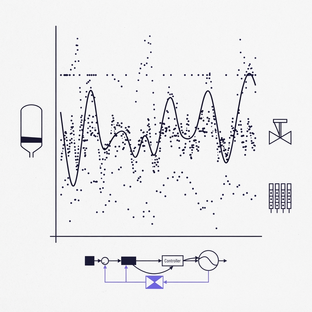
Search for neural controlled differential equations for irregular time series and you get the paper. You get its arXiv page, its NeurIPS proceedings PDF, its GitHub repository, and a conference tutorial that teaches it. All of that is correct and none of it answers the question most people arrive with, which is whether this method survives contact with a process that is still running.
That gap matters because the answer is not a straight yes. There is a specific property of the standard formulation that rules it out of live prediction entirely, and it sits in a follow-up paper that does not rank for the phrase at all. This article covers the mechanism, what the benchmarks actually measured, and the interpolation decision that determines whether the model can be used in a loop or only over a saved dataset.
Irregular sampling is the normal case, not the exception
Two things go wrong with real measurement streams, and they are different problems. A series is irregularly sampled when the gaps between observations vary. It is partially observed when some channels are missing at a timestamp where others are present.
The canonical example in this literature is medical. The PhysioNet sepsis dataset used in the original Neural CDE paper holds 40,335 ICU stays with 5 static and 34 time-dependent features, and only 10.3% of values are observed. That is not a corrupted dataset. That is what an intensive care record looks like, because tests are ordered when a clinician wants them.
A plant instrument stream has the same shape for different reasons. Sensors sit on different cadences by design, some because they are cheap and fast and some because they involve a sample and a delay. Channels drop out during maintenance and come back. Some measurements are event-triggered rather than periodic. The usual fix is to resample everything onto a common grid and forward-fill the holes, which works, and which quietly throws away the fact that a gap was there at all.
What a neural controlled differential equation actually changes
The problem with an initial condition
Neural ordinary differential equations are an appealing way to model something continuous, but they have a structural limitation that the Neural CDE authors state bluntly: the solution to an ODE is determined by its initial condition, and there is no mechanism for adjusting the trajectory based on subsequent observations. Set the model running and it evolves on its own. New data has nowhere to enter.
For a classification task over a fixed series that is tolerable. For anything where measurements keep arriving, it is fatal.
The data becomes the control path
The resolution comes from controlled differential equations, a piece of mathematics that predates the machine learning interest in it by decades. Instead of the hidden state evolving under its own vector field alone, it evolves driven by a path built from the data. Interpolate the observations into a continuous path X, and the model integrates the learned vector field against dX rather than against dt. Changes in the data change the local dynamics.
The framing the authors use is worth keeping: a Neural ODE is the continuous analogue of a ResNet, and a Neural CDE is the continuous analogue of an RNN. The hidden state is the same object an RNN carries, now defined at every instant rather than at each step.
Two consequences follow, and both are practical rather than aesthetic. First, the messiness of the data is pushed into the interpolation step, which is a far better place for it than inside the model architecture. Irregular spacing, missing channels and variable lengths all become properties of X, and the network itself never sees them. Second, because the differential equation is never interrupted to absorb an observation, adjoint backpropagation works across observations, giving an overall memory footprint of order L plus H rather than L times H, where L is the time horizon and H the vector field's memory.
The reference implementation and the torchcde library ship an example for exactly the awkward case, handling variable-length inputs, irregular sampling and missing data without any change to the model definition.
What the benchmarks measured, and what they do not tell you
The headline result is a robustness one. On the CharacterTrajectories dataset, the authors dropped 30%, 50% and 70% of observations at random and found that Neural CDE accuracy stayed roughly constant across all three, while every comparison model degraded as the drop fraction rose. It did so using an order of magnitude less memory than the alternatives. On the sepsis task, the Neural CDE produced the best AUC overall when observational intensity was supplied as a signal, and every model performed substantially worse without it.
That second finding deserves a moment. Observational intensity means the rate at which measurements were taken is itself informative: a patient being measured often is a patient somebody is worried about. On a plant the equivalent signal exists whenever sampling is not purely periodic, and the standard resample-and-fill pipeline destroys it.
The IJCAI-25 survey of neural differential equations for time series consolidates the wider picture across model families, with forecasting benchmarks run at 30%, 50% and 70% missingness and classification on the same sepsis data. Its conclusion is consistent: the advantage of these methods is most pronounced under irregular sampling, and it comes with lower memory use than conventional baselines.
Here is what none of that establishes. Every one of those tasks is offline. The whole series is available before the model runs. A controller does not have that.
The property that decides whether it runs on a live process
Natural cubic splines are not causal
This is the most useful thing on the page and it is not on the first page of results for the keyword.
The original Neural CDE interpolates with natural cubic splines. A natural cubic spline is fitted to the whole series at once, so any segment of the control path depends on every data value, including values after the point you are evaluating. The follow-up paper on the choice of interpolation scheme for Neural CDEs makes the consequence explicit: current implementations rely on non-causal interpolations, which is fine when the whole series is observed in advance, but means Neural CDEs are not suitable for online prediction tasks. A prediction at time t is quietly reading data from t plus one.
If you took the standard recipe and put it in a control loop, it would look like it worked in backtest and could not be deployed.
Rectilinear and Hermite controls
The same paper fixes it. It sets out four conditions a control path should satisfy, being adapted measurability, smoothness, boundedness and uniqueness, and then introduces two schemes that meet them. Cubic Hermite splines with backward differences join adjacent points with a spline whose gradients match the backward finite difference, which is smooth and depends only on data already seen. Rectilinear controls go further, advancing time and feature channels separately in a lead-lag fashion, and are the only scheme that is continuously online.
The recommendations are stated per case. Use rectilinear controls when the problem is online and needs a continuously online solution, or when it is online and has missing data. Use cubic Hermite with backward differences when the problem is online without missing data, or when it is offline, where it performs in line with the others at better speed. Keep natural cubic splines only when the task is offline and speed matters more than accuracy. The authors are candid about the cost: rectilinear controls are typically slow and can carry high memory usage, but in many online cases they are the only option. Both new schemes are implemented in torchcde.
The online benchmarks were three continuous monitoring tasks from MIMIC-IV, beating ODE baselines on all three. Continuous monitoring of a system whose state you cannot fully observe is a reasonable description of a cultivation basin or a reactor, minus the regulatory weight.
Choosing between a NODE, an NCDE and an NSDE
The three families answer different questions, and the CIKM-25 tutorial on neural differential equations frames the split cleanly around assumptions, strengths and limitations.
Reach for a neural ODE when you want continuous hidden-state evolution and the input arrives once. Reach for a neural CDE when an external signal drives the dynamics and keeps arriving, which is the case for any instrumented process. Reach for a neural SDE when the uncertainty is part of what you are modelling rather than noise to be smoothed away.
Two open problems from the survey are worth carrying into a deployment decision rather than discovering later. Adaptive integrators can produce unpredictable computation times in stiff regions, which is an uncomfortable property for anything with a deadline. And stability guarantees, which exist for neural ODEs and CDEs through Lipschitz constraints, remain incomplete for neural SDEs.
What it costs once the model has to answer on time
A model whose inference time depends on the stiffness of the region it is integrating through is not automatically compatible with a control budget. Fixing that is a separate engineering job from fitting the model, and it is the part that decides whether any of this reaches a plant.
At Equation Labs the numbers from our own control stack are these. Growth-model accuracy of R-squared above 0.95, a safety layer answering in under 2 ms, and end-to-end edge latency of 285 ms reduced from 1.2 seconds, validated on a 500 L pilot basin with zero safety violations across 400 simulated years, as published on our research page. The accuracy figure is the modelling result. The latency figures are what made it deployable, and they came from a different discipline: compressing that model to hit a latency budget, and choosing correctly between distillation and quantization rather than applying both by reflex.
Two further steps sit between a fitted continuous-time model and a controller you would trust on live equipment. One is sim-to-real transfer, because a model validated in simulation has not yet met the sensor noise, the actuator lag or the drift. The other is a hard safety layer, typically control barrier functions, because a learned model that is right on average is still not permitted to be wrong at the wrong moment.
Derive the equations first. Then decide what runs them.
FAQ
What is the difference between a neural ODE and a neural CDE?
A neural ODE trajectory is fixed by its initial condition, with no mechanism to adjust on later observations. A neural CDE drives the vector field with a continuous path interpolated from the data, so each new observation changes the local dynamics. Informally, a neural ODE is the continuous version of a ResNet and a neural CDE is the continuous version of an RNN.
Can a neural CDE make predictions in real time?
Not in its standard form. Natural cubic spline and linear controls are non-causal, so a prediction at a given time depends on data not yet observed. Rectilinear controls are the only scheme that is continuously online, and cubic Hermite splines with backward differences are online in the discrete sense when no data is missing.
How much missing data can it tolerate?
In the original handwriting benchmark, accuracy stayed roughly constant with 30%, 50% and 70% of observations dropped, while comparable models fell away. The sepsis benchmark ran with 10.3% of values present. Tolerance depends on whether the missingness is random or structured, but the method is built for the regime rather than patched for it.
Do I need to resample my sensor data onto a fixed grid first?
No, and doing so works against the method. The continuous-time embedding absorbs non-uniform spacing and absent channels directly. Resampling and forward-filling discards the timing pattern, which the sepsis results suggest can be informative in its own right.
Which library should I use?
torchcde, released alongside the original paper, with the rectilinear and Hermite-with-backward-differences controls added by the later interpolation work.