
Safe reinforcement learning with control barrier functions is the one branch of safe RL that offers something stronger than a preference. A reward penalty makes an unsafe action expensive. A barrier function makes it inadmissible. That difference is why the method reaches proposals for controllers that act on live equipment, and why it is worth being precise about what the guarantee says.
It is a conditional statement. The safe set stays invariant provided four things hold: you have a model accurate enough to differentiate, the input can actually reach the constraint everywhere it matters, the controller runs fast enough that continuous-time reasoning survives discretisation, and the optimisation has a feasible answer at every step. Each of those has a documented failure mode in the literature. This article is about the four conditions rather than the theorem, because on a plant the theorem is the easy part.
What a control barrier function actually guarantees
Safety is written as a scalar function of state. A survey of learned control barrier functions and their use in reinforcement learning states the construction compactly: safety is associated with a continuously differentiable function h(x), the system is safe where h(x) is at least zero, and the safe set C is the zero superlevel set of h. Maintaining safety means making C forward invariant, which is the property that gives the method its force. Start inside the set and you stay inside the set, indefinitely.
The naive route to that, insisting the derivative of h never goes negative, is too strict to be useful. It forbids the system from ever spending safety margin, which forbids most of the work you wanted it to do. The usable condition instead allows h to decrease at a rate that shrinks as you approach the boundary, scaled by an extended class K function. Far from the boundary you may move quickly toward it. Close to it you may not.
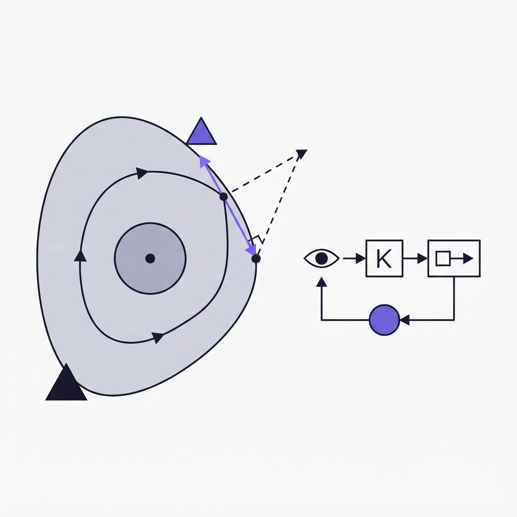
For a control-affine system this condition is linear in the input, which is the whole reason the method is practical. Given a nominal action from any controller, including a learned policy, you solve a quadratic program that finds the admissible input closest to the one proposed. Quadratic programs of this size solve in real time. So the safety layer is a projection: the policy asks, the barrier condition defines the feasible set, and what reaches the actuator is the nearest point in it.
Three properties follow, and they are the reason people reach for this rather than a shield built from an enumerated state abstraction. The guarantee is about set invariance rather than about the policy, so it is indifferent to which RL algorithm sits upstream. It is mission agnostic. And it is cheap enough to run in the control loop rather than as an offline check.
Filter at deployment, filter in training, or both
Everything above describes a runtime filter. There is a second place to put the same machinery, and choosing between them is the first real architectural decision.
The runtime case is made most concretely by work on acceleration-based CBF-QP enforcement on real robot hardware. The filter wraps a pre-trained policy and constrains it onto the safe set at runtime without modifying training at all. On a 19-DoF humanoid, a policy that had already been trained with safety constraints embedded still produced 10.04 constraint violations per second on real hardware. Adding the runtime filter reduced that by 92 percent, to 0.80. On a 7-DoF manipulator it eliminated violations entirely. The gap between a policy trained to be safe and a policy prevented from being unsafe is not rhetorical, and that number is what it looks like measured.
The same paper names the reason training-time safety alone was insufficient: methods that embed constraints during learning provide distributional guarantees, and those degrade under distributional shift, which is exactly the regime a deployed system spends its life in. It also names the operational advantage. Because the filter is a post-processing layer, a safety requirement that appears after training, a new collision constraint from online perception for example, can be added without retraining anything.
The counterargument is put well by CBF-RL, which applies the filter during training instead. Its objection is that a policy which never sees the constraint never learns it, so it keeps proposing actions that get corrected, and the resulting behaviour is conservative. Filtering rollouts during training, combined with a barrier-inspired reward term, gives the policy direct corrective supervision: it observes what it proposed, how the filter changed it, and what that cost. The claim is that the constraint is then internalised well enough to deploy without a runtime filter, which matters when the platform has tight real-time and compute limits, because a runtime filter means solving an optimisation program at every single control step.
The AAAI architecture that put barrier functions into end-to-end safe RL is the in-training variant of the same idea, with a model-free RL controller, model-based CBF controllers and online Gaussian process learning of the unknown dynamics, giving a guarantee that holds with high probability throughout learning. A related line frames safety as a differentiable robust CBF layer inside model-based RL, so the gradient passes through the safety layer and exploration is steered by it rather than merely censored by it, with modular reward learning that supports zero-shot transfer.
There is no general answer. What decides it is whether your deployment states resemble your training states. If they do, in-training filtering buys you a cheaper control loop. If they do not, and on an industrial process they usually do not, the runtime filter is the only thing standing between an out-of-distribution state and the actuator. Our own stack keeps the filter in the loop for that reason, which is a separate question from what has to be proven before a learned policy moves a valve.
Assumption one: a model accurate enough to differentiate
The barrier condition contains Lie derivatives of h along the system dynamics. You cannot evaluate it without a model. As the survey puts it, basic CBFs are model-based and need prior knowledge of both agent and environment, which is precisely what compromises the guarantee under model uncertainty.
Work on disturbance-observer-based CBFs with residual model learning makes the useful distinction, which is that model error is not one thing. There is internal error, meaning your nominal dynamics are wrong in their parameters or missing physics, and there is external disturbance, meaning fast-changing effects the model was never going to contain. They call for different instruments. Residual model learning handles internal error well, learning the discrepancy between predicted and actual next state, but it fails on fast external disturbance. A disturbance observer handles the fast case, but if the nominal model is also badly wrong the observer has to absorb everything at once and its estimate converges slowly. Combined, each covers the other's blind spot. Validated on a physical racing car, which is a fair test precisely because the model changes as the vehicle does.
The engineering question that follows is diagnostic rather than architectural. Which error dominates on your plant. On a thermochemical process where the feedstock composition varies between deliveries, most of the error is internal and slow. On an outdoor cultivation basin, weather is a genuine external disturbance and the two sources are comparable. That determination is cheap to make from historical data and expensive to skip, because it decides which of these two instruments you build.
Assumption two: uniform relative degree, which almost nobody checks
This is the failure mode that ranks lowest on the search results page and matters most in integration.
Relative degree is which time derivative of the output the control input can directly influence. A first-order CBF safety filter requires that degree to be one across the entire domain. Work on preventing inactive CBF safety filters caused by invalid relative degree assumptions points out that this is a local property of a nonlinear system and need not be constant over its domain, that the assumption is frequently overlooked in practice, and that higher-order CBFs relax the value but still assume it is uniform.
Where the assumption fails, the Lie derivative of h along the input dynamics goes to zero. The barrier constraint becomes redundant. The filter does not report an error and does not refuse; it degenerates into projecting the proposed input onto the static admissible input set, which is to say it stops doing its job while continuing to run. Large and possibly unsafe inputs pass through untouched. In a discrete-time implementation the symptom is chattering near the safety boundary, and then constraint violations.
Sit with what that means for validation. An inactive filter and a satisfied constraint produce the same log line. Every step shows the certified input equal to the proposed input, which reads as a well-behaved policy that never needed correcting. The paper's mitigation is a safety filter built from multiple CBFs, synthesised so that at least one remains active everywhere on the boundary, demonstrated in simulation and then on a real quadrotor where a single-CBF filter produced chattering and safe set violations and the multi-CBF version did not. The instruction to carry into any integration is smaller than the theory: instrument whether the constraint is binding, not only whether it is satisfied.
Assumption three: the proof is continuous time and your plant is sampled
The invariance argument is written in continuous time. Real controllers apply inputs at discrete instants and hold them, because computation and communication take time. The same authors treat this directly: real-world systems form a sampled-data system under zero-order hold, and this worsens the relative degree problem, because an input that is feasible at the sampling instant persists for the entire interval and can carry the state past the boundary before the next decision.
Two routes exist. Discrete-time CBFs enforce safety directly in discrete time but often produce a nonconvex optimisation, which costs the computational tractability that made the method attractive. Or you keep the continuous-time formulation and adjust for sampling, either by tightening the barrier condition for a fixed interval or by adapting the interval online through self-triggering. Both work by bounding how far the true trajectory can deviate from the last sampled state. Taking the fixed-interval route yields something a project can actually specify: an upper bound on sampling time for guaranteed safety, derived from the Lipschitz constants of the dynamics and the policy.
That bound is a hardware requirement wearing a theorem's clothes, and it is where a great deal of published safe RL stops being deployable. The figures from our own control stack are these. The safety layer answers in under 2 ms. End-to-end edge latency is 285 ms, reduced from 1.2 seconds.
The asymmetry between those two numbers is deliberate. The safety layer runs two orders of magnitude faster than the policy it guards, because a filter that queues behind a late policy cannot overrule it. Hitting the 285 ms figure at all was a separate discipline from the modelling, a matter of compressing the model until it fits the budget rather than hoping the hardware would be enough. And the sampling bound is one-directional in a way that is easy to misread: satisfying it is necessary for the guarantee, not sufficient, because it assumes the model those Lipschitz constants came from.
Assumption four: the quadratic program has to have an answer
Every guarantee above is stated over a non-empty admissible set. Input constraints are real: actuators saturate, valves have travel limits, and the set of admissible inputs is a bounded polytope rather than all of R^m. Intersect that polytope with the barrier condition near the boundary and it can come back empty. The hardware paper is explicit that its forward-invariance guarantees hold under feasibility and bounded modelling error, and both halves of that clause are load-bearing.
So a defined fallback is not optional, and it is not a machine learning artefact. It is an interlock: a predefined action, a controlled shutdown, or a handover to the existing base regulatory layer, specified before the first policy is trained and owned by whoever carries the operational risk. If your safe RL architecture has no documented answer for the case where the QP is infeasible, it does not have a safety story yet, it has a safety story for the states where nothing went wrong.
There is a performance clause worth stating in the same place, because it is what people fear about filters. Task performance is untouched while no constraint is binding; the nominal RL objective is preserved in violation-free regimes. When a constraint does bind, what the filter minimises is a design choice with consequences. Minimising deviation in commanded effort and minimising deviation in the resulting motion are different objectives that produce different safety-performance trade-offs, and picking one by default is picking one without knowing.
What changes when the process is slow and alive
Almost every result cited here comes from robotics: manipulators, quadrotors, humanoids, a racing car. Fast, well-instrumented, cheap to reset. The reasoning transfers. The operating point does not.
A cultivation basin runs on hours and days rather than milliseconds, which sounds easier and is not. Slow dynamics mean a bad action is not visibly bad for a long time, so the barrier has to be evaluated against a predicted trajectory rather than an immediate response. Observability is worse: concentration, health and composition are inferred from optical and spectral proxies rather than measured, so h(x) is evaluated on an estimate that carries uncertainty a joint encoder does not. And the failure is not recoverable on the next cycle. A crashed culture restarts on the same timescale as the growth it interrupted.
Our recorded figures for that setting, on the same research page, are growth-model accuracy at R-squared above 0.95, validated on a 500 L pilot basin with zero safety violations across 400 simulated years. The simulated years are the honest part of that sentence and should be read as what they are: coverage of the state space, not elapsed operating time. What makes them worth something is the record around them. On the OptiVX programme, 29 accounted work phases and 400 simulated years certified, which is the difference between a contract research programme and a demonstration.
Two pieces sit either side of this one. The irregular, multi-rate measurement problem underneath h(x) is a modelling decision, and continuous-time models built for irregular sampling exist for exactly it. And between a filter that holds in simulation and a filter that holds on the plant sits sim-to-real transfer, which is where the model in assumption one gets tested rather than assumed.
Derive the equations first. Then decide what is allowed to act on them.
FAQ
Is a control barrier function the same thing as a safety shield?
Same family, different instrument. Both are hard-constraint methods, meaning they actively alter the agent's action during exploration rather than discouraging unsafe behaviour through reward, which is what separates them from soft-constraint approaches that offer no explicit guarantee. The barrier function is the control-theoretic member of that family, working through forward invariance of a safe set for a control-affine system, and it is what you use when the dynamics are continuous and differentiable rather than enumerable as an abstraction.
Do I have to hand-design the barrier function?
Usually, and it is the acknowledged bottleneck. Synthesising a CBF is not straightforward and requires ample domain knowledge, and there is no a priori knowledge of the largest safe set associated with a given safety specification, so a hand-crafted barrier is typically more conservative than it needs to be. That is the motivation for the data-driven branch of the field, which learns barrier functions from system data or from expert demonstration.
Can I add a CBF filter to a policy that is already trained?
Yes, and it is one of the strongest practical arguments for the runtime approach. A QP safety filter constrains any pre-trained policy at runtime without modifying training, which also means constraints can be changed or added at deployment without a retraining cycle.
Does a CBF still work if my state estimate is noisy?
Only if the uncertainty is carried explicitly, and then the guarantee changes character. Modelling the unknown dynamics with a Gaussian process gives a probabilistic guarantee, one that holds with high probability rather than absolutely. A disturbance observer covers the fast external component. Neither restores the deterministic statement, and a validation record that quotes the deterministic one while running on estimated state is overclaiming.
Which comes first, the barrier function or the reward?
The barrier function, and by a wide margin. It has to be expressible in physical units without reference to the learning objective, because the whole point is that it constrains any policy you put upstream. If your safety property cannot be written down without mentioning the reward, there is no barrier to synthesise.