
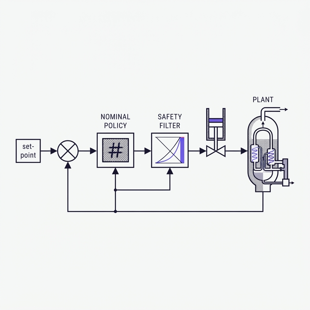
A control barrier function safety filter is a component, not a proof. You already have a controller. It works, it is task-oriented, and it is not necessarily safe, which is the exact phrasing a comparative review of backup-based filters uses for the nominal policy every one of these methods wraps. The filter goes between that policy and the actuator and minimally modifies what passes through.
The theory of why this works is settled and written up elsewhere, including in our own account of what a control barrier function actually is. What is not written up anywhere is the installation, which is four decisions in order: which filter family, how aggressive, inside what time budget, and instrumented how. This article is those four.
The integration surface is smaller than the theory
The filter does not need your policy. It needs the control-affine dynamics, the barrier, and the input limits.
That is visible most concretely in working code. The cbfpy configuration asks for the state and control dimensions, optional control limits, the functions f and g, and the barrier h declared at the correct relative degree. Then the loop reads the state, calls the nominal controller, and passes its output through a single filter call before applying it. The policy above the call is untouched and does not know the filter exists.
That is the property worth buying. A constraint discovered after deployment gets added by editing h, not by retraining anything.
What a runtime filter is worth, measured
The strongest available evidence comes from robotics, where violations are countable. An acceleration-based CBF-QP filter wrapped around pre-trained RL policies was tested on real hardware. A policy that had already been trained with safety constraints embedded still produced 10.04 constraint violations per second on a 19-DoF humanoid. The filter reduced that by 92 percent, to 0.80. On a 7-DoF manipulator it eliminated violations entirely. Task performance of the RL objective was preserved in violation-free regimes, which is the answer to the fear that a filter makes the controller worse: it does nothing at all until a constraint binds.
The honest counter-position is that you may not need it at runtime. CBF-RL enforces the barrier during training instead, on the argument that a policy with no knowledge of the CBF keeps proposing corrected actions and ends up conservative, and reports deployment without an online filter. The decision between them is one question. Do your deployment states resemble your training states? On a plant with seasonal feedstock and drifting sensors, they do not, and the runtime filter is the only thing between an out-of-distribution state and the actuator.
Four families, and choosing between them is a scheduling decision
The word "filter" covers four distinct constructions with different compute profiles. Work on set-based safety filters for industrial constrained systems lays out three of them against the requirement set that actually matters industrially: certified constraint satisfaction, predictable online computation, and a transparent tuning interface.
Set-based filters verify containment in a precomputed invariant set. They scale favourably with state and input constraints, but they intervene abruptly at the set boundary and carry no recovery mechanism.
CBF-based filters bound the change of a scalar barrier and give smooth, tunable intervention. The cost is synthesis: a scalar barrier that stays valid across a complex intersection of constraints either scales poorly or buys tractability with conservatism.
Predictive filters solve a receding-horizon problem at every step and define the invariant set implicitly. Maximum flexibility, substantial online computation.
The fourth family is backup-based, and the comparative review unifies it: certify the current action by showing the system could switch to a known backup manoeuvre, stay in the safe set, and reach a terminal invariant set. Backup CBF, Model Predictive Shielding and gatekeeper are all this, and the review shows MPS is a special case of gatekeeper.
None of these is correct in general. What decides it is what the control period can afford, which is the next section.
One parameter sets how intrusive the filter is
The reason the CBF formulation keeps winning integrations is that its aggressiveness is one number with a physical reading.
With a linear class-K choice, that number s lives in the interval from zero to one, and the motor-drive study is explicit about what it does: at s equal to 1 the filter is a permissive invariance check, and as s approaches zero it becomes a damped, early-intervention supervisor. Smaller values produce earlier and smoother intervention. It is set at commissioning, by someone watching the closed loop, without touching the safe set geometry that was computed offline.
Compare that with the predictive branch, where intervention aggressiveness is tuned indirectly through cost weights, horizon length and terminal set, all solved online. Same behaviour available, no single dial.
There is a second choice hiding in the quadratic program itself, and defaults conceal it. The hardware paper above formulates alternative objectives, minimising deviation in commanded torque or minimising deviation in induced acceleration, and calls them principled control over the safety-performance trade-off. They are different objectives. Choosing neither is choosing one.
The budget the filter has to fit inside
This is where published safe control stops being deployable, so use numbers.
On a permanent-magnet synchronous motor drive, the explicit set-based implementation evaluated in a mean 14.5 microseconds at s equal to 1, rising to 23.7 microseconds at s equal to 0.5, with a theoretical worst case of 28.04 microseconds across all 127 regions, inside a 150 microsecond sampling window. That leaves 121.96 microseconds for ADC and PWM. The important word is not the magnitude, it is deterministic: the explicit law is region localisation followed by affine evaluation, so the worst case is bounded rather than hoped for.
Getting there means not calling a solver. Work on closed-form expressions for CBF-based safety filters states the obstacle plainly, which is that off-the-shelf QP solvers are a problem wherever control actions must be computed at very high frequency, and partitions the state space so each region has an algebraic solution. Its resource-aware implementation detects when the state leaves a region and only then recomputes the active set, which turns a per-step solver call into an occasional one.
Our own stack sits at a different scale and keeps the same asymmetry. The measured figures are a safety layer answering in under 2 ms against an end-to-end edge latency of 285 ms, reduced from 1.2 seconds. Two orders of magnitude between the guard and the guarded, deliberately, because a filter that queues behind a late policy cannot overrule it. Reaching the 285 ms was its own discipline of compressing the model until it fits the budget, not a hardware purchase.
Conservatism is the failure you will actually meet
Infeasibility gets the attention, and it belongs with the assumptions the guarantee rests on. In commissioning, the problem is almost always the opposite: a filter that intervenes when it did not have to, so the plant underperforms and the operator switches it off.
The backup-based review names the mechanism exactly and calls it safety evaluation on backup. Safety is judged along the backup trajectory rather than along continued execution of the nominal policy, so the filter can override an input that would have stayed safe. A state can fail the validity test for an early switch even though running nominal a little longer would have reached a state from which the backup is valid. The fix is searching over switching times rather than fixing one, which is what gatekeeper does, and the review is equally clear that too short a horizon or too coarse a search grid collapses gatekeeper back into MPS.
The predictive branch reaches for a different lever, and work on approximate predictive control barrier functions is unusually honest about its price. Hard constraints frequently go infeasible under unmodelled dynamics or sensor noise, so constraints get softened with slack variables, and that generally loses the theoretical properties as soon as the system does violate a constraint. Its own decrease hyperparameter can be relaxed to reduce interventions after the barrier is learned. Softening is a decision about what your certificate says, not a numerical convenience.
Instrument the inactive set, not the violation count
A log of zero violations proves nothing on its own. It is equally consistent with a well-tuned filter and with one that intervenes constantly.
The quantity that separates them is the filter-inactive set: the states where the nominal input already satisfies every constraint and passes through unchanged. The comparative review uses it precisely because it measures intrusiveness rather than safety, and it is cheap to log. Record the intervention rate, which constraint was active, and the barrier margin at intervention. Those three turn a filter from an assertion into a record, which is what has to be proven before a learned policy moves a valve.
Our figures on the cultivation side read that way: growth-model accuracy at R-squared above 0.95, validated on a 500 L pilot basin with zero safety violations across 400 simulated years. The simulated years are coverage of the state space, not elapsed operating time, and should be quoted as such.
What changes when the process is slow
Every microsecond figure above comes from fast, well-instrumented hardware. A cultivation basin or a thermochemical stage moves on hours, and the risk moves with it.
The solver stops being the constraint. The barrier is evaluated on an estimate rather than a measurement, because concentration and composition are inferred from optical and spectral proxies. A bad action is not visibly bad for hours, and the failure does not reset on the next cycle. All of that pushes the uncertainty back into the model the Lie derivatives came from, which is tested rather than assumed in sim-to-real transfer.
Derive the equations first. Then decide what is allowed to act on them.
FAQ
Does a CBF safety filter slow the control loop down?
Measured rather than argued: 28.04 microseconds worst case inside a 150 microsecond sampling window on a motor drive, and deterministic because the explicit law reduces to region localisation plus affine evaluation. The variable cost is the online solver call, and the closed-form partitioned implementation removes it for most steps by recomputing only when the state leaves its region.
Can I add a safety filter to a policy someone else trained?
Yes, and it is the normal case. The filter needs the control-affine dynamics, the barrier and the input limits, not the policy weights or its training history. What it does not need is a retraining cycle, which is why a constraint that appears after deployment can be added without touching the policy.
If I already run MPC, do I need a separate safety filter?
Only for the tuning interface and the compute profile. A predictive safety filter is a legitimate family in its own right, but aggressiveness is then tuned through horizon length, cost weights and terminal set, all of which are solved online, rather than through one parameter fixed at commissioning against a safe set computed offline.
What does softening the constraints with slack variables cost?
The theoretical properties, generally, from the moment a constraint is actually violated. It is standard practice because hard constraints go infeasible under unmodelled dynamics and sensor noise, but it changes the class of statement your validation record is allowed to make.
How aggressive should the barrier parameter be at first commissioning?
Start permissive and tighten while watching the intervention rate. The permissive end behaves as a plain invariance check that only acts at the boundary; tightening moves the filter toward an early-intervention supervisor with smoother behaviour and a modestly higher evaluation cost. Tune it against the inactive set, not against the violation count.