
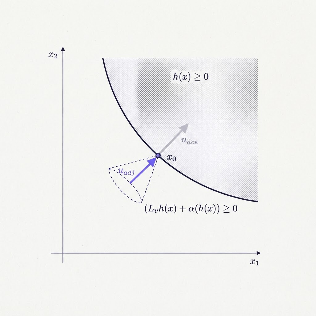
A control barrier function is a scalar function of the system state whose sign tells you whether you are safe, and whose derivative tells you which control inputs are still allowed. That is the whole idea. Everything else is bookkeeping around it.
Most explanations of control barrier functions are written for someone about to prove a theorem. This one is written for someone about to put a filter in a control loop, so it covers the same definitions with the same precision and then keeps going into what the method costs, what it demands of your model, and where it quietly stops working.
What a control barrier function is, in one paragraph
Write safety as a continuously differentiable function h(x). The safe set C is the region where h(x) is at least zero, which makes C the zero superlevel set of h. The goal is not to reach a point but to never leave a region, a property called forward invariance: start inside C and stay inside C, for all future time.
That framing is deliberate. The canonical survey of control barrier functions traces the notion of safety to Leslie Lamport's 1977 work on program correctness and pairs it against liveness. Liveness says good things eventually happen, and asymptotic stability is its control-theoretic instance. Safety says bad things never happen, and set invariance is its instance. The survey's argument is that safety received far less attention than liveness because the Lyapunov function dominated the study of the latter, and that the control barrier function is meant to play for safety the role the Lyapunov function plays for stability.
Why the obvious version of the idea does not work
The first safety filter almost everyone builds is a conditional. A quadcopter case study in a netted flight arena writes it out honestly: if the drone's x position is outside the bounds, set the commanded x velocity to zero, and the same for y and z. It reads as obviously correct and it is not. The check only fires once the state is already outside the box, and at that point zeroing the velocity command does not undo the momentum that carried it there. A filter that acts at the boundary acts too late.
The theoretical version of the same mistake is to demand that h never decreases. That forbids the system from ever spending safety margin, which forbids most of the work you wanted it to do. Approaching a wall at all becomes inadmissible even from across the room.
The fix is to let h decrease, but at a rate that shrinks as you approach the boundary. The original CBF quadratic program paper makes exactly this move, allowing the barrier function to grow when it is far from the boundary rather than insisting its derivative never be positive, and notes that this greatly increases the set of admissible barrier functions. The modern statement scales the allowed decrease by an extended class K function of h. Far from the boundary you may move quickly toward it. Close to it you may not. The survey adds the property that makes this more than a convenient relaxation: for compact sets the condition is necessary and sufficient, so it is minimally restrictive. You are not trading safety for permissiveness. You are stating the least restrictive condition that still implies invariance.
The condition, and why it is linear in the input
In words: the rate of change of h along the closed-loop trajectory must be at least minus alpha of h, where alpha is that class K function.
Evaluating it requires Lie derivatives of h along the system dynamics, which is the first thing to notice about the method. A model is not optional. It is the object you differentiate.
The second thing to notice is what happens for a control-affine system, where the dynamics split into a drift term and an input matrix multiplying u. The barrier condition then becomes affine in the control input. A course chapter on certificate functions draws the consequence out: for control-affine systems you can synthesise a controller satisfying these constraints by solving a quadratic program, a convex problem class that solves efficiently in practice. An affine constraint plus a quadratic cost is a QP, and QPs of this size run inside a control loop. That single structural fact is why control barrier functions left the literature and reached hardware.
From certificate to controller: the CBF quadratic program
The deployed shape of the method is a filter with three parts.
A nominal controller proposes an action. It can be a PID loop, a trajectory tracker, a human operator's setpoint or a learned policy. The barrier condition defines the set of inputs that keep the safe set invariant from the current state. The QP returns the admissible input closest to the one proposed.
The framing that matters here is minimal invasiveness: the filter wraps a possibly unsafe nominal feedback policy and is imposed as a runtime constraint, altering the command only when the command needs altering. While no constraint binds, the nominal controller's behaviour is untouched.
Note what the guarantee attaches to. It is a statement about the set and the dynamics, not about the upstream controller. The filter does not care what proposed the action or how it was trained, which is why the same construction shows up in collision avoidance for multi-robot systems, motion planning and robotic manipulators, and why it is the standard way to put a hard constraint around a learned policy. The failure modes of that particular combination are a longer subject, treated separately in the four assumptions underneath the guarantee.
Control barrier function vs control Lyapunov function
Both are certificates, and the course chapter's parallel is the cleanest way to hold them apart. A control Lyapunov function certifies that a system can be stabilised by some admissible control. A control barrier function certifies that a safety constraint can be maintained by some admissible control. One is about eventually arriving, the other about never leaving.
Because both produce constraints affine in the input for a control-affine system, they compose into a single QP. The design decision inside that composition is the load-bearing one. The journal treatment of CBF-CLF quadratic programs makes safety a hard constraint and relaxes the stability objective into a soft one carrying a penalty, so that safety and stability never need to be simultaneously satisfiable. When they conflict, performance yields and the resulting control law is still provably Lipschitz continuous. The same paper contrasts this with invariance control, which enforces derivative conditions on the boundary of the set and yields discontinuous control laws that can chatter, in the manner of sliding mode control.
That is the difference between a method that survives integration and one that does not. Any safety scheme that requires the safety constraint and the performance objective to be jointly feasible has no defined behaviour on the day they are not.
The worked example everyone starts from
Adaptive cruise control is the example the field converged on, because it contains all three ingredients in a form anyone can picture. The performance objective is to reach and hold a desired cruising speed. The safety constraint is a minimum following distance behind the lead car, the half the speedometer rule. The physical limits are bounded acceleration and braking force.
The simulation in the ACC paper is worth reading for its second case rather than its first. Running the QP with only the speed objective and the following-distance barrier, the vehicle converges exponentially to the desired speed until the lead car is close, then matches its speed and holds the safe distance. Correct behaviour on the constraint that was encoded. But the acceleration and braking force limits, which were not encoded, are violated during both acceleration and braking. Adding a second barrier function for the force constraints fixes that, and the cost is visible: convergence to the desired speed is slower, braking begins earlier, and the following distance is more conservative throughout.
Read as a lesson rather than a result, it says two things. Constraints you did not write down are not enforced, however obviously physical they are. And each constraint you add buys safety with performance, in a quantity you can see in the trajectory rather than argue about.
The three things the explainers leave out
The tutorial literature is explicit about its own open problems, and the survey of practical challenges in safe control synthesis lists three.
Finding a valid barrier function at all is not trivial. Writing down a function whose superlevel set is the region you care about is easy. Establishing that the barrier condition can be satisfied everywhere in that region under your dynamics and your input limits, which is what makes it a control barrier function rather than merely a constraint function, is not. This is why an entire branch of the field is devoted to synthesising CBFs offline, searching for the condition's parameters, or adapting them online until the candidate becomes valid.
High relative degree and input constraints compound each other. Relative degree is how many times you have to differentiate h before the control input appears. When it exceeds one, the basic condition is empty at the first derivative and you need Higher Order CBFs. When actuator limits are also present, the class K functions in that construction stop being a tuning choice and start determining the size and shape of the admissible set, so they have to be chosen deliberately. Input Constrained CBFs generalise the higher-order construction for exactly this case, and can also handle systems whose relative degree is not uniform across the domain.
The model you differentiate is wrong. Modelling and parametric uncertainty is named as the third challenge, and it forces robust, adaptive or learning-based formulations if the guarantee is to mean anything off the nominal model. There is a fourth limitation in the same list that is easy to miss and honest to state: the input a CBF produces is only pointwise optimal, often called myopic. It is the best admissible action now, with no account taken of where the trajectory goes next. That is the real trade against a predictive method, and it is a matter of control barrier functions against model predictive control rather than of theory.
What the filter costs in the loop
The QP solves at every control step, so the filter has a latency budget, and it has to be faster than whatever it guards. A safety layer that queues behind a late policy cannot overrule it.
The measured figures from our own control stack show the asymmetry that requirement produces. The safety layer answers in under 2 ms. End-to-end edge latency is 285 ms, reduced from 1.2 seconds. Two orders of magnitude between them is not an accident of implementation, it is the specification. Hitting the 285 ms number was its own discipline, a matter of compressing the model until it fits the budget rather than assuming the hardware would cover it.
The same stack records growth-model accuracy at R-squared above 0.95 and validation on a 500 L pilot basin with zero safety violations across 400 simulated years. The simulated years should be read as what they are, coverage of the state space rather than elapsed operating time.
Sampling deserves one more sentence, because the invariance argument is written in continuous time and no real controller runs in continuous time. This is not a private worry: preserving safety under zero-order hold and under output feedback appear in the practical-challenges paper as named implementation problems, alongside the theory.
Where this sits if you are building one
Write the safety property in physical units first, without reference to any controller or reward. If it cannot be stated that way, there is nothing to certify yet.
Then check the relative degree of that property against your actuator, because it decides whether you need the basic construction or a higher-order one. Then decide where the filter lives, at runtime around a nominal controller or inside training, and instrument whether the constraint is binding rather than only whether it is satisfied. Then confirm the model those Lie derivatives run on holds outside simulation, which is the business of sim-to-real transfer, and that your state estimate is good enough to evaluate h on, which for irregularly sampled processes means continuous-time models built for irregular sampling.
The build order is the same one that governs what has to be proven before a learned policy moves a valve, and the mechanics of the wrapper itself are the subject of how a control barrier function safety filter is built.
Derive the equations first. Then decide what is allowed to act on them.
FAQ
Is a control barrier function the same as a barrier function in optimization?
Shared ancestry, different object. Barrier functions were first used in optimization, where they penalise approach to a constraint boundary. A control barrier function is a Lyapunov-like certificate on a control system: because h's derivative depends on the input, the condition becomes an inequality constraint on u whose satisfaction implies forward invariance of the safe set. The optimization version shapes a cost. The control version restricts an action.
What does forward invariance mean in plain terms?
If the state starts inside the safe set, it never leaves it, for all future time. It is a different kind of promise from asymptotic stability, which says trajectories converge to an equilibrium and says nothing about the path they take getting there. A system can be perfectly stable and still pass through a state that destroys it.
Do I need a model to use a control barrier function?
Yes, and this is the most common thing to underestimate. The barrier condition contains derivatives of h along the system dynamics, so it cannot be evaluated without dynamics to differentiate. Model uncertainty is therefore not an edge case but one of the three named open challenges in the field, and it is what robust, adaptive and learning-based CBF formulations exist to absorb.
Is a CBF filter conservative?
Somewhat, and by construction. It is pointwise optimal, choosing the best admissible input now without accounting for the future trajectory. Every additional constraint you encode also costs performance, visibly: the adaptive cruise control simulation brakes earlier and follows further back once actuator force limits are added as a second barrier. Online parameter tuning and predictive formulations exist specifically to claw some of that back.
Where are control barrier functions actually used?
The application domains named in the survey literature are automotive systems, multi-robot systems, quadrotors and walking robots: fast, well-instrumented, cheap to reset. Slow industrial and biological processes are a much smaller literature, which is worth saying plainly. The mathematics transfers unchanged. The operating point, where a bad action is not visibly bad for hours and the state is inferred rather than measured, does not.