
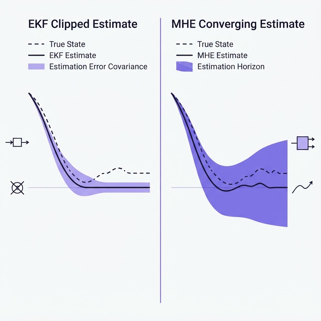
The moving horizon estimation vs Kalman filter question usually arrives late in a project. A model exists, some states have no sensor, and a controller is about to act on an estimate of them. The Kalman filter is the reflex choice because it is recursive, cheap and optimal in one well defined setting. Moving horizon estimation (MHE) is the alternative that keeps being recommended in the process control literature and keeps being avoided in practice because it solves an optimisation problem at every sample.
This article reads the primary sources so you do not have to. It answers three questions in order: when the two estimators are literally the same thing, under what conditions the extended Kalman filter fails even with a perfect model, and what MHE charges for not failing. It closes with the case that decides the matter for us, a living system whose states cannot go negative and whose measurements arrive at wildly different rates.
What the two estimators actually compute
The Kalman filter: a recursion that is optimal in one setting
The Kalman filter is the optimal state estimator for an unconstrained linear system driven by normally distributed state and measurement noise. The Rawlings and Lima lecture notes lay the mapping out as a table: linear model plus Gaussian noise gives you the Kalman filter; a nonlinear model plus Gaussian noise gives you the extended Kalman filter (EKF); add inequality constraints or general noise to either and the answer becomes MHE. The same notes name the price in one line: an online solution to a quadratic or nonlinear program.
Everything the Kalman filter knows about the past is compressed into a mean and a covariance. That compression is exact for the linear Gaussian case and is the reason the filter is a handful of matrix operations per step. It is also the reason it cannot take an inequality constraint. There is no place in a Gaussian for the statement "biomass is never below zero".
Moving horizon estimation: an optimisation over a window
MHE starts from a different question. Given the last N measurements, which trajectory of states and disturbances is most consistent with both the model and the data? Rao, Rawlings and Lee explain why this reformulation is forced rather than chosen: once inequality constraints on states or noise are added to a linear estimation problem, recursive solutions such as Kalman filtering are no longer available, and the problem written as a quadratic program grows with every new measurement. The moving window exists to bound the problem size. Only the most recent N samples are optimised, and everything older is summarised in a single penalty term on the first state of the window, the arrival cost.
That structure is what makes MHE the natural partner of model predictive control. Both solve a finite horizon optimisation at every step, both carry a model forward in time, and both accept constraints as constraints rather than as afterthoughts. We cover that pairing from the control side in our comparison of a control barrier function vs model predictive control.
Where they are the same estimator
For an unconstrained linear system with a quadratic objective, the arrival cost can be computed exactly from the Kalman filter covariance and moving horizon estimation reduces to Kalman filtering. The Processes 2020 review of nonlinear estimation for chemical and biochemical processes makes the same point from the Bayesian side: for an unconstrained, linear, infinite horizon problem the least squares solution and the recursive solution coincide because minimising squared error is maximising the Gaussian conditional density.
So the comparison is never "which is more accurate" in the abstract. On the problem the Kalman filter was built for, they return the same number and the Kalman filter returns it faster. The question is only what happens when the problem leaves that setting.
Where the extended Kalman filter fails with a perfect model
Multiple steady states and a poor initial guess
The reference for this is still the 2002 technical report by Haseltine and Rawlings, later published in Industrial and Engineering Chemistry Research. Its design is the reason it is still cited: both estimators get exactly the same information, the same tuning parameters, model and measurements. The EKF is not handicapped. It is simply asked to do the job on reaction systems with hard constraints.
The report shows that even with perfect concordance between model and plant, the nominal EKF can fail to converge to the true state when two things hold at once. The model and measurement admit multiple states that satisfy the same steady state measurement, and the estimator is given a poor initial guess. Given a poor estimate of the initial state, the EKF cannot reconstruct the evolution of the state while MHE can. Given an even poorer estimate, both fail, which is the honest half of the result.
Clipping is not a constraint
The second half is what happens when physical knowledge is added. The authors constrain the concentrations to lie between 0 and 4.5 in both estimators. With that information MHE converges to the true states while the clipped EKF estimates are trapped on the constraint. Relaxing the bound to 5.5 does not free the EKF. Clipping a Gaussian estimate back inside a bound after the fact is not the same as estimating under the bound, because the covariance that drives the next update still believes the state was outside.
The report also records the failure mode on the MHE side. If the estimation horizon is too short, the MHE estimates are pinned against the state constraint, and increasing the horizon remedies the problem. The authors read this as the data in a short window being unable to overcome the bias of the arrival cost approximation. Keep that sentence; it is the whole tuning problem in one line.
What moving horizon estimation costs
An optimisation at every sample
The Rawlings and Lima notes are candid about this: MHE is robust to modelling errors but requires an online optimisation, and both MHE and particle filtering need more user experience to set up and more computational resources to run. The Processes 2020 review adds that computational cost for large scale industrial processes is still a challenge, because a nonlinear program must be solved at every time step. Our own engineering view of what fits inside a sample interval, and why the number is often tens or hundreds of milliseconds rather than seconds, is in the article on a bioreactor control strategy.
The arrival cost is an approximation
For anything nonlinear or constrained, the arrival cost has to be approximated, and the choice is not cosmetic. Qu and Hahn note that the common approach is a first order Taylor expansion of the model followed by an EKF covariance update, and show that computing the arrival cost with an unscented Kalman filter instead gave a lower mean squared error for every horizon length and noise level they tested, with the advantage shrinking as the horizon grows. Ungarala is blunter: the formulation of the arrival cost is in general an ad hoc procedure, the EKF based covariance used to weight it can diverge even in higher order implementations, and a poorly formulated arrival cost forces large horizons, which in turn hinder fast real time estimation.
Note the irony. The Kalman filter you were trying to replace comes back inside MHE as the device that summarises the past. Valipour and Ricardez-Sandoval studied exactly this on a wastewater treatment plant and a polystyrene process under nonlinear MPC and concluded that an appropriate arrival cost method such as the EKF is adequate to keep large, challenging systems in closed loop. The two estimators are collaborators more often than rivals.
How long the horizon has to be
Qu and Hahn give the two rules of thumb that circulate in practice. The horizon should not be shorter than the number of system states, and Rao and Rawlings recommend twice the order of the system. Their own case study with a non-negativity constraint on a concentration shows mean squared error falling as the horizon moves through lengths of 3, 4, 6 and 10, with the gain per extra sample diminishing. A longer window costs more per solve. A shorter one risks the pinned estimates Haseltine and Rawlings saw.
Measured compute from two real systems
Two studies put numbers on the trade. A vehicle positioning study in Sensors ran a nonlinear constrained MHE with a gradient descent solver on a dSpace real time system at a 100 ms sample time, with a fixed maximum iteration count so the real time constraint is met even when the optimum is not reached. Against it, a square root EKF had a computational time up to 20 times lower. The same EKF failed as soon as a single sample of measurement delay was introduced, while the MHE absorbed delayed and out of sequence satellite fixes by placing them where they belong inside the window.
On a process, Tuveri and colleagues implemented MHE on experimental data from a fed-batch cultivation of Corynebacterium glutamicum. With a 60 second update interval and a 30 minute horizon, the optimisation solved in 0.05 to 1 second, well inside the interval. The compute objection is real for large plants and small sampling intervals. For a cultivation sampled every minute it is not an objection at all.
Why living systems tilt the comparison toward MHE
Non-negative states and multi-rate measurements
The Tuveri study is also the clearest statement of why biology changes the answer. Their estimator carries a hard lower bound of zero on all four states to avoid infeasible concentrations. An EKF or UKF has to reach for clipping or a separate optimisation to achieve the same, and time varying parameters have to be appended as extra states with no way to bound them. Then there is sampling. An absorbance probe reads every 10 seconds while a sugar measurement by HPLC arrives every 30 to 60 minutes. A window of past data has a natural slot for a late, slow measurement; a recursive filter has to be patched to accept one.
Those two features, states that cannot be negative and measurements that arrive on different clocks, describe every cultivation we have worked on. They are also why our sibling article on physics-informed neural networks for state estimation in bioprocesses treats the estimator and the model as one design problem rather than two.
Model mismatch and the hybrid architecture
Tuveri's honest finding cuts the other way: simple tuning could not fully compensate for unmodelled dynamics, and model mismatch produced steady state offsets. MHE is robust to model error, not immune to it. The Processes 2020 review describes the architecture that practitioners converge on when compute is tight and constraints matter: a hybrid in which an EKF provides fast estimates between less frequent MHE solves and the MHE corrects the EKF when it drifts, demonstrated on a recombinant protein process in E. coli. That is the same division of labour as the arrival cost story, made explicit.
What we measured on a 500 L pilot basin
Our own work sits on this fault line. In the OptiVX programme the control stack was validated on a 500 L pilot basin with a growth model whose accuracy reached an R-squared above 0.95. The estimator feeds a safety layer that runs in under 2 ms, and end to end edge latency was brought from 1.2 seconds to 285 ms. Over 400 simulated years of operation the safety layer recorded zero violations. Those numbers set the budget. A state estimate that respects non-negative biomass and multi-rate sensing is only useful if it lands inside the sample interval on the hardware at the basin, which is why the horizon length and the solver iteration cap are chosen against a latency figure, not against an accuracy figure alone.
A decision procedure
| Your situation | Use | Why |
|---|---|---|
| Linear model, no constraints, roughly Gaussian noise | Kalman filter | MHE returns the same estimate at higher cost |
| Mild nonlinearity, no constraints, compute very tight | EKF or UKF | Recursive; the vehicle study found the EKF up to 20 times cheaper |
| States with hard bounds, multiple steady states, uncertain initial state | MHE | Clipped EKF gets trapped on the bound; MHE converges |
| Measurements at different rates or arriving late | MHE | The window has a slot for them; the EKF failed at one sample of delay |
| Constraints matter but the sample interval is short | Hybrid EKF plus MHE | EKF between solves, MHE to correct and to supply the arrival cost |
The sibling questions each get their own article: Kalman filter for state estimation for the recursion itself, extended Kalman filter vs Kalman filter for what linearisation costs, and Kalman filter alternatives for particle, unscented and learned estimators compared on one process.
FAQ
Is moving horizon estimation always more accurate than a Kalman filter?
No. For an unconstrained linear system with Gaussian noise the two produce the same estimate and the Kalman filter is cheaper. MHE gains only where the problem leaves that setting: hard constraints, non-Gaussian noise, multi-rate or delayed measurements, or a poor initial guess combined with multiple steady states.
What is the arrival cost in moving horizon estimation?
It is the penalty on the first state of the window that stands in for all measurements older than the window. For a linear unconstrained system it is exact and comes from the Kalman covariance. For anything else it is an approximation, usually an EKF or UKF covariance, and a poor approximation either biases the estimates or forces a longer horizon to dilute it.
Can MHE run in real time on edge hardware?
Within limits set by the sample interval. A gradient descent MHE with a fixed iteration cap ran at 100 ms on a dSpace real time system, and a fed-batch cultivation MHE solved in 0.05 to 1 second against a 60 second interval. Fast processes with many states still favour a recursive filter or a hybrid.
Does MHE replace the Kalman filter inside model predictive control?
Usually not. In practice an EKF supplies the arrival cost or the fast estimates between MHE solves, and the MHE and the nonlinear MPC share the same moving horizon structure, so the controller's initial condition comes from an estimator built the same way it is.