
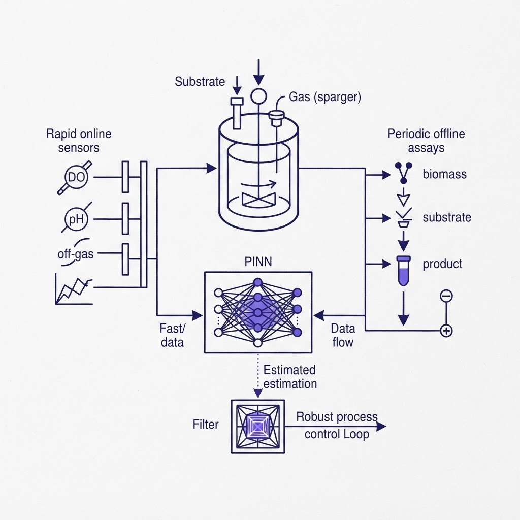
Physics informed neural networks for state estimation in bioprocesses solve a problem every fermentation and cultivation engineer recognises. The variables that decide the batch, biomass, substrate and product concentration, are read from offline assays hours apart. The variables that arrive every second, dissolved oxygen, pH, off-gas, temperature, are not the ones you want to control. Something has to bridge the two, and the bridge has to be trusted enough that a controller can act on it.
A physics-informed neural network (PINN) is one candidate for that bridge. The pages that currently rank for the phrase are journal PDFs written for peers. This article reads them for a practitioner and answers three questions in order: which unmeasured states a PINN can actually infer from the probes you already have, how to test that before you train anything, and what the bioprocess studies measured when they tried.
The measurement problem a bioprocess actually has
The soft-sensing literature states the problem precisely. In a Pichia pastoris fermentation study, the three states the operator cares about, cell concentration, substrate concentration and enzyme concentration, cannot be measured directly. Three other outputs can. A virtual subsystem is placed between them so that the measurable three stand in for the unmeasurable three, and the training targets for that virtual sensor come from offline laboratory assays.
That is the whole shape of the problem. The states you control are sampled slowly and destructively. The signals you have are fast and indirect. Any monitoring scheme needs, in the words of a metabolic-informed soft-sensing paper, accurate real-time measurement of the important variables, and the important variables are exactly the ones without a probe.
Two features of production make this harder than a textbook CSTR. Fed-batch remains the dominant mode for biotherapeutics, and a hybrid-modelling study of recombinant Pichia notes that the nonlinear, high-cell-density character of these runs limits purely mechanistic models because parameter estimation and unforeseen biological interactions degrade their reliability. The equations are known in form and wrong in detail. A black-box model has the opposite failing: right wherever it has seen data, unconstrained everywhere else.
What a physics-informed neural network changes
One network, the balance equations in the loss
The cleanest definition comes from the paper that ranks first for this topic, Velioglu and colleagues in Computers and Chemical Engineering. In a PINN the deep network is the sole prediction model. It is informed about the governing physical laws during training through additional terms in the loss function. Feed it time and the batch conditions, and it returns the state trajectory. The mass balances are not solved numerically at run time; they are penalised at training time, so the network learns a trajectory that both fits the assay points and satisfies the balances between them.
For a bioprocess the practical consequence is that the physics does the interpolating. The assay gives you biomass at hour 0, 8, 16 and 24. The balance equation tells the network what biomass is allowed to do in between, and how it is coupled to the substrate it consumes and the oxygen it draws. The network no longer has to learn that coupling from data it does not have.
PINN versus hybrid model versus neural ODE
The same paper draws a line that is worth keeping. A hybrid model has distinct mechanistic and data-driven sub-models that jointly produce a prediction, the classic case being a mass-balance ODE with a neural network supplying the unknown kinetic rate. A PINN is better regarded as a special variant of a data-driven model trained with physical laws as constraints. One architecture integrates a known equation around a learned term; the other learns the whole solution and is punished for violating the equation.
A third relative, the neural ordinary differential equation, learns the vector field itself and integrates it forward. We have covered neural ordinary differential equations separately, and a mechanism-first explainer of how physics-informed neural networks work sits alongside this one. The choice between the three is not aesthetic. It decides what you can estimate, which is the next question.
Which unmeasured states a PINN can infer, and how to test it first
The estimability heuristic
The Velioglu paper is explicit about the hard case: states for which neither direct observational data nor constitutive equations are available. Not a state you measure rarely, but a state you never measure and whose rate law you cannot write down. The authors propose an easy-to-apply heuristic to assess whether estimation of such a state is possible before any training, and demonstrate it on a continuously stirred tank reactor and a liquid-liquid separator. Their finding is that PINNs can infer immeasurable states with reasonable accuracy even when the constitutive equation for that state is unknown, provided the remaining structure of the semi-explicit differential-algebraic system ties the hidden state to the measured ones tightly enough.
The engineering translation is a question to ask of your own balances. If the unmeasured state appears in the right-hand side of an equation whose left-hand side you do measure, there is a path from data to state. If it appears only in equations whose other terms are also unknown, no amount of network capacity will recover it. The heuristic formalises that reasoning on the structure of the equations, and it is the single cheapest piece of work you can do before committing to a PINN. The generic bioreactor PINN study from 2025 cites exactly this differential-algebraic heuristic as the tool for deciding whether a PINN can recover hidden states in a partially known system.
Why the bound sits on the parameters, not the network
The paper that Google autocomplete carries for this keyword is Jiang and colleagues on calibration-free PINNs for adaptive state inference in bioprocesses. Its framing is that existing PINNs rely on fully calibrated mechanistic models, which makes them brittle under parameter drift and when internal states cannot be measured. Their framework jointly estimates the key quality indicators and the unmeasurable internal states, and was validated on industrial penicillin fermentation across strains and processes as well as on simulated and chemical cases.
The finding that matters most for a practitioner is stated empirically: the accuracy of unmeasurable-state estimation is bounded by the accuracy of the physical model parameters. A larger network does not buy a better estimate of intracellular product if the yield coefficient in your balance is 15 percent off. That is why the calibration-free formulation treats the drifting parameters as something to infer alongside the state rather than something to fix beforehand, and it is the reason a PINN built on a textbook parameter set tends to look excellent on the batch it was tuned on and disappoint on the next strain.
What the bioprocess studies measured
A PHA culture with four states and four rates
Catalao and colleagues used a PINN as the model inside a model predictive controller for a mixed microbial culture producing polyhydroxyalkanoates. The architecture is instructive because it is small. One feed-forward network with 5 input nodes, time plus the initial conditions of the cycle, and 8 output nodes. Four of those outputs are state variables: active biomass concentration, acetate concentration in the liquid, ammonium concentration in the liquid and intracellular PHA content. The other four are the kinetic rates. The network estimates the rates it was never given an equation for, constrained by the balances it was.
A generic bioreactor with five balances and unknown kinetics
The 2025 bioreactor PINN study takes the structure a step further with a dual-network design. The material balances of 5 state variables are encoded in the loss, while the reaction kinetics are deliberately excluded and left to be learned. The authors benchmark this against the general hybrid semiparametric bioreactor model under comparable prior knowledge across 2 case studies. In the first case the experiments followed a central composite design, with 9 runs used for training and 6 for validation. That is a small dataset by deep-learning standards, and it is the point: with the balances in the loss, the data only has to pin down the kinetics.
The paper is also honest about the limit. The extrapolative advantage of the PINN over the hybrid model that appeared in the first case study is not guaranteed in the more complex second case. Physics in the loss helps the network stay plausible outside the training envelope, but it does not make a wrong or incomplete balance right.
Industrial penicillin across strains
The Jiang calibration-free study is the only one of the three validated on an industrial dataset rather than a laboratory or simulated culture, and the only one that tests across strains and process variants. That cross-strain extrapolation is the test a production engineer actually cares about, because the model that works on one seed lot is not the problem. The reported robustness to noise and parameter variability under that validation is what earns the method a place in the discussion of real plants, and the parameter-accuracy bound above is the caveat that comes with it.
Where the PINN stops and the filter starts
A PINN is a model. State estimation, as the Velioglu paper reminds its readers, is classically the business of a filter: an algorithm that combines a model prediction with incoming measurements and weights each by how much it trusts them. The Kalman filter is the canonical example, and the paper notes that filtering techniques have recently been combined with PINNs for exactly this purpose.
For a living process this division of labour is the right one. The PINN supplies a physically consistent prediction of biomass or product between assays. The filter corrects that prediction every time a dissolved-oxygen or off-gas reading arrives, and corrects it hard every time an assay result lands. The PINN is what makes the model term in the filter good; the filter is what keeps it honest against drift the network never saw. How to do that without losing the filter's guarantees is the subject of a companion piece on hybrid Kalman filter and neural network state estimation. When the states carry hard constraints, non-negative biomass, substrate that cannot exceed the feed concentration, the comparison of moving horizon estimation versus the Kalman filter becomes the relevant one. If the term itself is new to you, start with what a soft sensor is, because a PINN wrapped in a filter is one.
What an estimator has to deliver before a controller may act on it
An estimate that is only used for a dashboard can be approximately right. An estimate that a controller acts on has to be accurate, fast and bounded, in that order, and those are measurable properties.
Our own cultivation control work gives a concrete reference for what the numbers look like when they are met. The continuous-time growth model governing the system reached a measured accuracy of R-squared above 0.95, validated on a 500 L pilot basin. The safety layer that screens every control action responds in under 2 ms. End-to-end edge latency, from measurement to actuated decision on the hardware at the basin, was brought down from 1.2 s to 285 ms, and the stack ran with zero safety violations across 400 simulated years, all documented at Equation Labs. Those figures describe the growth model and its control stack, not a PINN in particular; what they establish is the bar. An estimator whose error is unknown cannot feed a controller with a safety case, because the safety layer has to know how wrong the state might be.
That is also why the estimator and the controller are designed together. The architecture of a bioreactor control system sets which states the controller needs and at what rate, and that determines which hidden states the estimator must recover and how often. The same PINN that estimates the state can serve as the fast surrogate inside the optimiser; we cover that use in physics-informed neural networks inside model predictive control.
A build order that avoids the usual failure
The usual failure is a network trained on everything available, reporting a beautiful fit on held-out time points from the same batches, that collapses on the first new strain. The studies above, read together, give a build order that avoids it.
- Write the balances first, with the unknowns marked. List every state, every rate term, and label each rate as known, known-in-form or unknown. The Catalao and 2025 bioreactor architectures both start here: balances in the loss, kinetics left to the network.
- Run the estimability check before training. Apply the differential-algebraic heuristic to the marked balances. If an unmeasured state has no path to a measured one, add a measurement or drop the ambition. This is an afternoon of algebra that saves weeks of tuning.
- Decide what to do about parameters. Either calibrate them on data you trust and accept the Jiang bound, or treat drifting parameters as quantities to infer alongside the state. For anything that will see more than one strain, the second is the defensible choice.
- Split the data by experiment, not by time. The 2025 study held out whole central-composite runs, 6 of 15, rather than later time points of the same runs. Only that split tells you whether the model generalises to conditions it has not seen.
- Validate against the assay, not the probe. The targets are the offline laboratory measurements, as in the Pichia soft-sensing setup. A model that reproduces the online probes has reproduced the inputs.
- Wrap it in a filter before it touches a controller. The PINN predicts; the filter corrects and carries the uncertainty. Measure the residual against every new assay and set the controller's constraints from that residual.
- Measure latency on the target hardware. An estimator that runs in a notebook has not been built yet. The 285 ms figure above was measured at the edge, and a cultivation loop that needs a decision every few seconds has a budget to meet.
Treat the extrapolation caveat in the bioreactor study as the rule rather than the exception: physics in the loss narrows the space of wrong answers, it does not remove them. The estimator earns trust the same way any instrument does, by being checked against a reference, repeatedly, on the process it is installed on.
FAQ
Can a PINN estimate a state that has no sensor and no kinetic equation?
Under conditions, yes. The Velioglu study addresses exactly this case, states with neither observational data nor constitutive equations, and proposes a heuristic on the structure of the differential-algebraic system to decide beforehand whether such a state is estimable. It then shows reasonable-accuracy inference of immeasurable states on a CSTR and a liquid-liquid separator. If the heuristic says no, more data from the same probes will not change the answer.
Is a PINN the same as a hybrid semiparametric bioreactor model?
No. A hybrid model has separate mechanistic and data-driven parts, typically a mass-balance ODE with a network supplying the unknown rate, and solves the ODE numerically. A PINN is a single network that predicts the states directly and is trained with the balances as loss terms. The 2025 bioreactor study benchmarks the two under comparable prior knowledge and finds the PINN's extrapolation advantage holds in the simpler case but is not guaranteed in the more complex one.
What limits the accuracy of a PINN state estimate in a fermentation?
The physical parameters, not the network. The calibration-free study by Jiang and colleagues finds empirically that the accuracy of unmeasurable-state estimation is bounded by the accuracy of the mechanistic model's parameters. Parameter drift between strains and batches is therefore the practical failure mode, which is why their framework infers the drifting parameters jointly with the states rather than fixing them in advance.
How much data did the bioprocess PINN studies train on?
Far less than a conventional deep network needs. The 2025 generic bioreactor study trained on 9 central-composite-design experiments and validated on 6. Putting the material balances into the loss means the data only has to determine the unknown kinetics, which is what makes the method usable on a process where each experiment is a multi-day batch and an assay.