
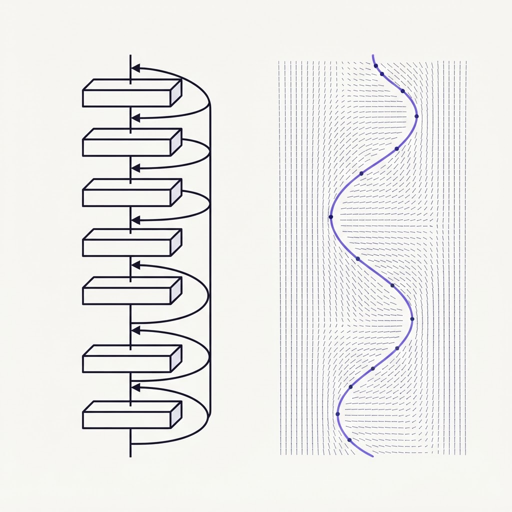
Neural ordinary differential equations, explained in one line: instead of training a network to predict the next value of something, you train it to predict how fast that something is changing, and let a numerical solver turn the rate into a trajectory. That is the whole idea. Most explainers then demonstrate it on handwritten digits, which is the one setting where the idea has the least to offer. This one uses a physical process, because that is where a model of the derivative stops being a curiosity and becomes the obvious thing to learn.
Neural ordinary differential equations explained in one sentence
The original paper by Chen, Rubanova, Bettencourt and Duvenaud put it precisely: rather than specifying a discrete sequence of hidden layers, parameterize the derivative of the hidden state using a neural network, and compute the output with a black-box differential equation solver. In symbols, the model is
dh/dt = f_theta(h(t), t)
h(T)  = h(0) + integral from 0 to T of f_theta(h(t), t) dt
The network f_theta never outputs the answer. It outputs a velocity: at this state, at this moment, move this way, this fast. The answer is whatever you get by following that velocity from a starting point for a given length of time.
Start with a process, not a picture of a digit
Take a heated water tank. Its state is a temperature. Its input is heater power. Physics tells you the shape of the story before you have any data: the temperature rises when you put energy in, falls toward ambient when you do not, and falls faster the hotter it is. What physics does not hand you is the exact form of every loss, lag and nonlinearity in a real vessel with real insulation and a real sensor bolted to its side.
There are two ways to learn this tank from logged data. The first is a discrete model: given the temperature now and the heater setting now, predict the temperature one sample later. It works until the logger skips a sample, or someone changes the sampling rate, at which point the model is answering a question it was never trained on. The second is to learn the rate of change: given the temperature and the heater setting, how fast is the temperature moving right now? That quantity does not care when you happen to measure. Integrate it for 3 seconds or 30 and you get a prediction for either.
That second model is a neural ODE. On a tank the choice is natural, because the tank really is a system whose state evolves continuously under a rule. On MNIST it is not, and the sceptics noticed. One of the clearest MNIST walkthroughs ends with its author not yet convinced the performance boost justifies the additional computation, and not sure why a continuous model should be closer to the truth for a classifier. That is a fair verdict on digits. It is the wrong verdict to carry over to a reactor, a battery or a bioreactor.
From residual layers to a continuous flow
A residual block is one Euler step
The bridge from ordinary deep learning is the residual network. A residual layer updates its state as h_next = h + f(h). Euler's method, the oldest way to solve a differential equation numerically, updates a state as h_next = h + step * f(h). Set the step to one and they are the same line of arithmetic, which is why a residual layer is one Euler step with its step size fixed and left implicit.
Stack many residual layers with small updates and you are taking many small Euler steps. Push the step toward zero and the stack becomes a smooth flow. At that point the network is no longer a list of layers. It is a single small network with one shared set of weights that reports the velocity of the state at any point and any time.
The solver decides the depth
Once the forward pass is a call to an ODE solver, decades of numerical analysis come along for free. Modern solvers adaptively choose step sizes and use high order approximations to cut the number of steps required. They take small careful steps where the trajectory bends and long strides where it is nearly straight.
The number of times the solver calls f_theta is called the number of function evaluations, or NFE, and it is the closest thing a neural ODE has to depth. Unlike a layer count it is not fixed: it is chosen per input, it can drift during training, and forward-pass time is proportional to it. The original paper frames this as a dial: you can explicitly trade numerical precision for speed.
For the tank, this means a quiet steady state costs almost nothing to simulate, and a sudden heater step costs more, because the solver has to work harder to follow the transient. Compute goes where the physics is doing something.
How a neural ODE is trained: the adjoint method
Constant memory, and where that number comes from
Training needs gradients of a loss with respect to the weights. The direct route is to record every operation the solver performed and backpropagate through all of them, which means storing the whole trajectory and every internal solver stage. Memory then grows with NFE, the very quantity you just made adaptive.
The alternative the paper used is the adjoint sensitivity method, an idea from 1960s optimal control. It defines a second ODE for how sensitive the final loss is to the state at each instant, and solves it backward in time from the end. The forward trajectory is thrown away and recomputed on the way back alongside the adjoint, in one combined reverse solve. On MNIST the paper measured the payoff: O(1) memory for the ODE network against O(L~) for backpropagating through the solver, where L~ is the NFE, and O(L) for an ordinary residual network.
The caveat the tutorials skip
That constant-memory trick rests on an assumption that most introductions never state. Re-solving the ODE backward to recover the forward trajectory implicitly assumes the integrator is reversible, and there are no reversible adaptive integrators for first-order ODEs. The DifferentialEquations.jl team, writing with one of the paper's authors, showed an equation where the backward solution with the Adams method had more than 1700% error in its final point, even with solver tolerances of 1e-12.
They also pointed out that adjoint sensitivity is not new: solver libraries such as CVODES shipped it in 2005, along with checkpointing schemes that save intermediate time points to make backward passes accurate, at the cost of some memory. The practical lesson for a physical model is simple. If your dynamics are sensitive or stiff, do not take constant memory as free. Check the gradients, or use a checkpointed adjoint, and spend the memory.
What a neural ODE cannot do
The flow view brings a hard limitation with it. Because the learned field gives one velocity at each point, two trajectories can never cross. A one-dimensional neural ODE cannot learn the map that sends -1 to +1 and +1 to -1, because the paths would have to meet at the origin. A residual network can, because its discrete jumps are allowed to leap over each other.
The standard fix is augmented neural ODEs: add a few extra state dimensions so trajectories that would collide have room to pass. One tutorial goes as far as to say that in general you should use augmented neural ODEs instead of vanilla ones, and points to second-order formulations for physical systems whose dynamics are naturally higher order, which is most mechanical ones.
For a physical engineer this limitation is less exotic than it sounds. If your measured state really is the full state of a deterministic system, its trajectories should not cross either. When a fit insists on crossings, it is often telling you the state is incomplete: an unmeasured temperature, a hidden concentration, a valve position nobody logged. Augmenting the state is then not a trick, it is admitting the missing variable.
Stiffness is the other wall. A process that mixes very fast and very slow dynamics forces an explicit solver into tiny steps everywhere. That is the argument for stiff-aware solvers inside the training loop, rather than whatever default ships with the tutorial.
Why the continuous view pays off on physical data
Three properties make neural ODEs worth their cost on a process rather than an image.
Irregular sampling stops being a problem. Because the model is a vector field, you can evaluate the solution at whatever times the sensors actually reported, and irregular time series become something a single shared dynamics can model. If samples are not just irregular but missing across channels, the formulation extends to neural controlled differential equations.
Accuracy on real dynamics is measurably higher. In a benchmark across nonlinear dynamical systems, Rahman and colleagues found neural ODEs reduced open-loop test error by two to three orders of magnitude against neural state space models, paid for with higher inference time per sample. That trade, and how to choose between neural ODEs and alternatives like SINDy, is the subject of our piece on neural ODEs for nonlinear system identification.
The learned model can be re-simulated. A neural ODE learns the vector field itself, so you can start it from a new initial condition or drive it with a new input sequence. A physics-informed neural network, by contrast, learns a solution tied to the initial conditions and inputs it was trained on. The same study found that Euler, RK4 and DOPRI5 reached comparable accuracy at very different training cost, so the most expensive solver is not automatically the right one.
From an explained model to a running controller
Understanding a neural ODE is the easy half. Getting one to run in closed loop on hardware is a different set of problems, and the figures from our own control stack at Equation Labs show where the effort goes. Growth-model accuracy reached R-squared above 0.95. That is the modelling result. End-to-end edge latency was reduced from 1.2 seconds to 285 ms, with a safety layer answering in under 2 ms, validated on a 500 L pilot basin with zero safety violations across 400 simulated years. Those are deployment results.
Each of the costs above shows up in that second set of numbers. NFE becomes latency, which is why compressing the model to hit a latency budget is its own discipline. A model fitted to logged data has not yet met sensor noise, actuator lag or drift, which is the work of sim-to-real transfer. And a model that is accurate on average is still not allowed to be wrong at the wrong moment, so the hard guarantees come from control barrier functions, not from confidence in the fit. If you want to build one yourself next, start with neural differential equations in Python.
FAQ
Is a neural ODE the same as a physics-informed neural network?
No. A neural ODE learns the vector field, the rule for how the state changes, so it can be re-simulated from new initial conditions and inputs. A PINN learns a solution to one specific initial value problem and needs detailed knowledge of the governing equations to guide training.
Are neural ODEs better than ResNets for image classification?
Not clearly. The main selling point on images is constant training memory, and careful practitioners remain unconvinced the continuous model is any closer to the truth for a classifier. The case for neural ODEs is strongest when the data really comes from a system evolving in time.
Which ODE solver should I use to train a neural ODE?
Start with an adaptive explicit solver for non-stiff dynamics and compare against a cheap fixed-step one; on an identification benchmark, Euler, RK4 and DOPRI5 reached similar accuracy at very different cost. If the process mixes fast and slow dynamics, switch to a stiff-aware implicit solver.
What is the number of function evaluations in a neural ODE?
It is how many times the solver calls the dynamics network during one forward pass. It plays the role of depth, but it is chosen per input by the solver's error control, so inference time varies with how hard the trajectory is to follow.