
Search this phrase and you get one paper. You get its arXiv abstract, its full HTML rendering, and its laboratory landing page, which is three results for a single benchmark. That benchmark is good and its headline is quotable: neural ordinary differential equations identify nonlinear systems more accurately than the alternatives by two to three orders of magnitude.
What no page on that results list does is turn the finding into a decision. If you have measurement data from a reactor, a tank cascade or a cultivation basin, and the model you fit has to end up inside a controller rather than inside a paper, the accuracy ranking is not the question. The question is which method your system actually permits, and what the accuracy costs you at the moment the controller has to answer.
The result that owns this phrase, and the part nobody quotes
The benchmark study compared neural ODEs against neural state space models and classical linear subspace identification across eight nonlinear dynamical systems, autonomous and non-autonomous, chaotic and non-chaotic. It measured three things rather than one: open-loop prediction accuracy, sensitivity to hyperparameters, and inference time.
The accuracy result is the one that travels. Open-loop test mean squared error was lower for the neural ODE than for the neural state space model on every system analysed, by a factor of roughly ten squared to ten cubed. Both nonlinear methods beat the linear subspace models, which is unsurprising, but the gap between the two nonlinear families is large enough to matter.
The second result is quieter and arguably more useful. The standard deviation of test MSE for the neural ODE was equal to or lower than that of the neural state space model across all systems, with the relative improvement reaching three orders of magnitude. In plain terms, the neural ODE reached a good model with far less hyperparameter searching. Anyone who has tuned a state space network knows what that saves.
The third result is the one that gets dropped from the summaries. Inference time per sample was higher for the neural ODE on eight of the nine systems. The typical penalty was a factor of 1.1 to 4.4. On the aerodynamic dataset it was a factor of about 50.
A fifty-fold inference penalty is not a footnote when the model is destined for a control loop. It is the constraint that decides whether the accuracy is available to you at all.
Why a continuous-time model suits a physical process
Parameterise the derivative, not the layer
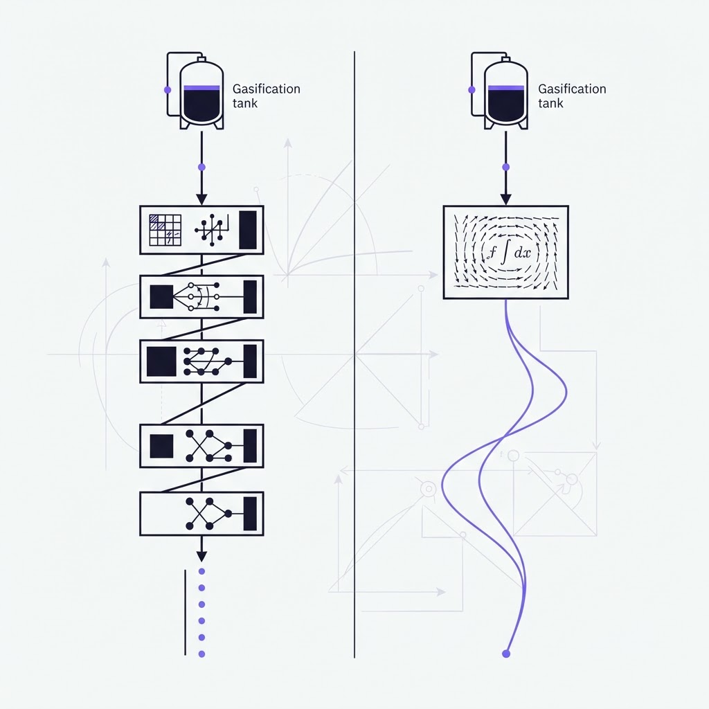
The original formulation replaces a discrete sequence of hidden layers with a network that parameterises the derivative of the hidden state. The output is then whatever a black-box differential equation solver returns for that initial value problem. Training works through the adjoint sensitivity method, which solves a second augmented ODE backwards in time, scales linearly with problem size, keeps memory cost low and gives explicit control over numerical error. Solutions exist and are unique wherever the network is Lipschitz continuous in the state, which holds for finite weights and ordinary nonlinearities.
For system identification this is not an architectural preference. A reactor, a heat exchanger or a growing culture is a continuous time-evolution process. A discrete-time model is an approximation of it chosen for convenience; a differential equation is the object itself. That alignment is where the accuracy gap in the benchmark comes from.
What the formulation buys in practice
Two consequences show up quickly on real measurement records.
The first is tolerance for how the data was collected. The benchmark noted that neural ODEs captured long-term transients on the vehicle system without any downsampling, which is exactly the preprocessing step that quietly destroys slow dynamics. Because a neural ODE integrates forward in time rather than estimating derivatives from finite differences, it also carries less stringent requirements on observation frequency than methods that must differentiate the data numerically before they can fit anything.
The second is that an adaptive solver spends computation where the dynamics demand it. That is a genuine advantage for stiff regions and, as the inference numbers above show, the reason the method is slow.
The comparison the benchmark did not run
The obvious missing competitor is sparse identification of nonlinear dynamics, SINDy, which fits a sparse combination of candidate functions and hands back a symbolic equation. A study on droop-controlled grid-forming units ran that comparison directly, and the result is more interesting than a winner.
SINDy produced the lowest median RMSE on all states, with low deviation across datasets. The authors then say something most method papers do not. They supplied the algorithm with a condensed set of candidate functions known to be part of the system dynamics, which in their own words renders the comparison almost unfair, and they add that using a larger set of more trivial candidate functions did not produce a good SINDy model at all. The neural ODE reached good prediction accuracy without any prior knowledge of the system's nonlinearities.
So the choice between them is not accuracy against accuracy. It is a bet about what you already know. SINDy is excellent when you can name the nonlinear terms in advance and merely need their coefficients. A neural ODE is what you use when you cannot, which on a real industrial or biological process is the more common situation.
Where each method breaks
SINDy and the full-observability requirement
A benchmarking study of SINDy across three nonlinear identification datasets is blunt about the failure modes: accuracy deteriorates in the absence of full state observability, and crafting an adequate library is hard in the presence of hard nonlinearities.
The numbers make the point better than the framing does. On the pick-and-place dataset, a plain linear autoregressive model with exogenous inputs outperformed the nonlinear models identified with the standard input-output SINDy approach. A neural network ARX reached 95.10 percent best fit rate against 93.24 percent for the best hands-on hidden-state SINDy variant, at the price of interpretability and higher hyperparameter sensitivity. The authors name full observability as perhaps the most limiting requirement of the method, with no definitive solution in the literature.
Partial observation is the normal condition on a plant. States are inferred, not measured. Anything you care about that sits behind a proxy sensor is a state SINDy cannot see.
The neural ODE and the arbitrary latent state
The neural ODE has a matching weakness in the opposite place. It is a black box, and it does not make reliable predictions outside the domain of its training region. Both limitations are documented, and both are the reason a family of structured and symbolic variants exists.
The subtler problem is what the latent state means. Work on structured Kolmogorov-Arnold neural ODEs evaluated black-box baselines on the Duffing and Van der Pol oscillators and on real F-16 ground vibration data, and found that the augmented neural ODE showed high variance and poor latent state interpretability, confirming a tendency to learn arbitrary latent representations, while a second-order variant produced stable but still non-interpretable trajectories. Only the structured model recovered latent coordinates corresponding to physical displacement and velocity, and it extracted the cubic stiffness of the Duffing system and the nonlinear damping of the Van der Pol system as symbolic expressions.
On a plant this is not an aesthetic complaint. An operator asked to accept a controller will ask what the model thinks the system is doing, and a latent vector with no physical meaning is a poor answer. A polynomial neural ODE attacks the same problem from another direction, using a network whose output is a polynomial transformation of the input so that a symbolic form can be recovered directly with symbolic algebra, without running SINDy on the trained model afterwards.
Choosing the instrument from what you already know
Three questions settle most cases, and none of them is about benchmark rankings.
Can you write down the candidate nonlinear terms? If yes, and the state is fully observed, a sparse or gray-box method will give you a compact equation and probably better accuracy. That is the easier problem and you should take the easier problem when it is on offer.
Is the state fully observed? If parts of it are inferred or measured indirectly, derivative-fitting methods are the wrong family, and the ARX result above shows how badly they can lose. A neural ODE that integrates forward does not need the derivatives.
Do you need an equation back, or a predictor? For control synthesis a predictor may be enough. For a certification file, a handover to a partner, or an argument with a process engineer, a symbolic form is worth accuracy. Structured variants sit in that middle ground.
One practical caveat on data volume. The benchmark's largest MSE reductions came on the continuous stirred-tank reactor and the two-tank systems, both carrying more than 10,000 data points, which it describes as the high-data regime among the datasets analysed. The advantage of the continuous-time model was clearest where measurement was plentiful.
The solver is part of the model
Two findings from the power system study are worth carrying into any identification campaign.
First, solver sophistication bought less than expected. Euler, fourth-order Runge-Kutta and DOPRI5 produced comparable one-step-ahead test MSE, with the adaptive solver only slightly ahead, while the training effort per epoch rose significantly for the more sophisticated schemes. Likewise, small networks with non-saturating and continuously differentiable activations such as softplus were preferable to larger ones.
Second, and more consequential, the learned model is closely tied to the integration method and the step size used during training, a property the literature calls baked-in discretization. It is beneficial as long as the sampling time of the data does not change, because it lets you deploy an accurate model with a lightweight solver. It is a liability the moment somebody re-rates a sensor or changes a logging interval.
That makes the plant's data acquisition rate a design decision taken at the start of the identification campaign, not an implementation detail settled later by whoever configures the historian.
From an identified model to a controller that answers on time
Return to the inference number. A model whose evaluation cost depends on the stiffness of the region it is integrating through has no fixed deadline, and a control loop is nothing but deadlines. Fitting the dynamics and making them run inside a cycle time are two separate engineering jobs, and the second one is where most continuous-time models stop.
The figures from our own control stack at Equation Labs, published on our research page, separate the two cleanly. Growth-model accuracy reached R-squared above 0.95. That is the identification result. End-to-end edge latency of 285 ms, reduced from 1.2 seconds, with a safety layer answering in under 2 ms, validated on a 500 L pilot basin with zero safety violations across 400 simulated years. Those are deployment results, and they came from different disciplines: compressing the model to hit a latency budget, and sim-to-real transfer, because a model validated against simulation has not yet met sensor noise, actuator lag or drift.
Two further pieces belong in the same picture. A learned model that is right on average is still not permitted to be wrong at the wrong moment, which is the job of a hard safety layer built from control barrier functions rather than from confidence in the fit. And if measurements arrive irregularly or channels drop out, the identification problem changes shape, which is the territory of neural controlled differential equations rather than the standard formulation described here. If you want the formulation itself before the selection problem, start with what a neural ODE is doing. If the resulting controller will be compared against a classical optimiser, the trade is set out in model predictive control.
Derive the equations first. Then decide what runs them, and how fast it has to answer.
FAQ
Is a neural ODE the same as a physics-informed neural network?
No. A physics-informed neural network learns the solution to an initial value problem, including the estimation of unknown parameters, so the result accounts for the specific initial conditions and inputs it was trained on and cannot be reused for simulation in a different setting. It also requires detailed knowledge of the underlying differential equations to guide learning. A neural ODE learns the vector field itself, which is what makes it reusable for closed-loop simulation and control synthesis.
How much data does a neural ODE need for system identification?
No minimum is established. In the eight-system benchmark, the largest reductions in open-loop error came on the continuous stirred-tank reactor and the two-tank systems, both with more than 10,000 data points, described as the high-data regime among the datasets tested.
Can a neural ODE give back a symbolic equation?
Yes, with a modified architecture. A polynomial neural ODE produces a polynomial transformation of its input, so a symbolic expression can be recovered directly through symbolic algebra rather than by applying a sparse regression method to the trained model afterwards. Structured Kolmogorov-Arnold neural ODEs extract compact symbolic expressions in the same spirit.
Which ODE solver should I train with?
Start simple. In the droop-controlled power system study, Euler, RK4 and DOPRI5 gave comparable test MSE while the higher-order schemes cost significantly more per training epoch. The more important point is that the solver and step size are baked into the learned model, so the choice cannot be revised freely once the model is fitted.
Will a neural ODE extrapolate outside the operating range it was trained on?
Not reliably. Standard neural ODEs do not make reliable predictions outside the domain of their training region, which is one of the two stated motivations for interpretable variants. For a physical plant this means the identification campaign has to excite the full range you intend to operate in, including the transitions, not only the steady states.