
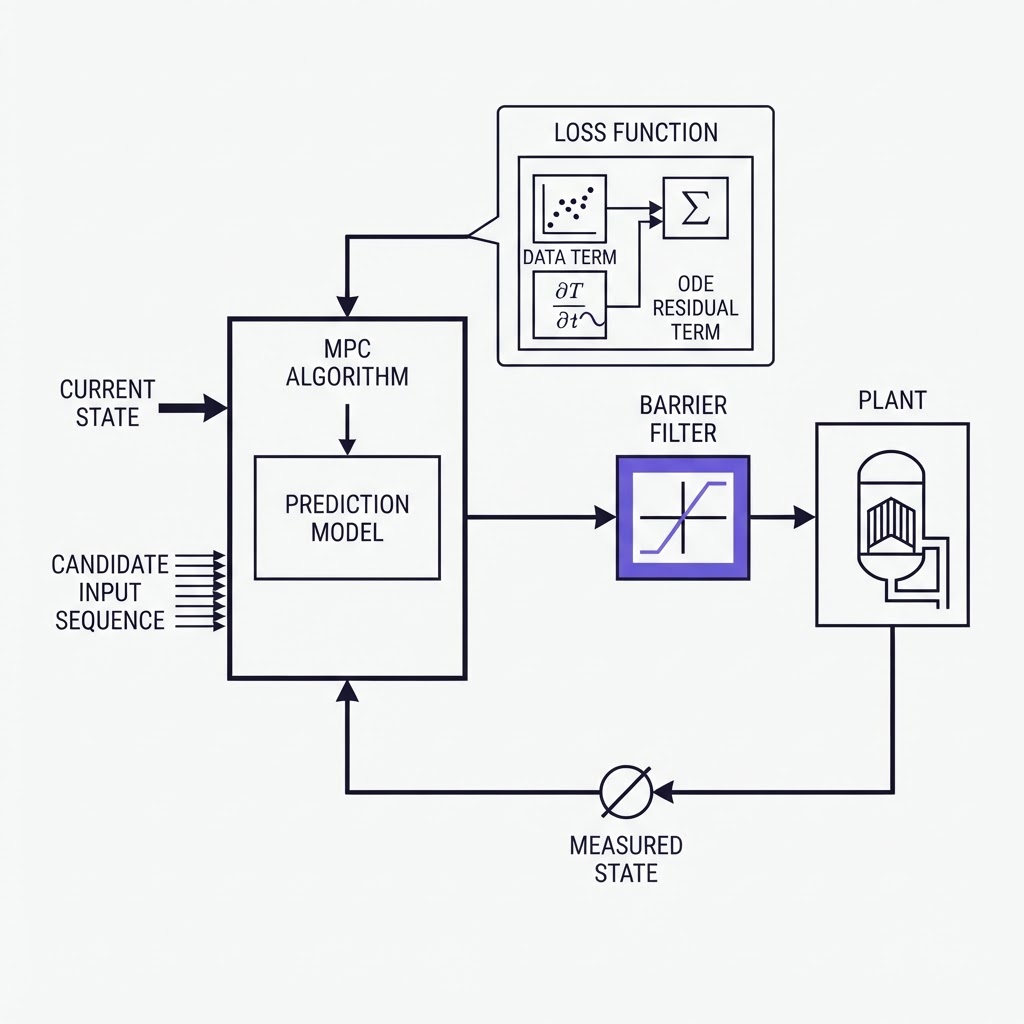
Physics informed neural networks for model predictive control solve one specific problem: the optimiser inside an MPC has to call its process model hundreds of times per control step, and the model that is accurate enough to trust is usually too slow to call that often. A PINN is a network trained to satisfy the governing equation as well as the data, so it can stand in for the numerical integration of that equation and answer in a single forward pass.
Everything ranking for this phrase is a journal paper proving the idea on one system. What those papers do not do is add up. This article does the adding: what the surrogate measurably buys, the structural change needed before a PINN can take a control input at all, the one benchmark that shows where it degrades, the one experiment where it closed the loop on a living process, and how we build it in our own control stack.
Why a predictive controller needs a surrogate at all
Model predictive control solves a constrained optimisation over a finite horizon at every step, applies the first move, and repeats. The quality of that plan is capped by the model underneath it, and so is the speed. The National University of Singapore group's 2023 paper in the Journal of Process Control states the bottleneck without hedging: what has prohibited real-time MPC on nonlinear processes is model representation and identification, and the development of accurate and computationally efficient process models remains the bottleneck. The same paper names the catch with the obvious fix. Machine learning models solve the speed problem, but their generalisation is contingent on the quality of the training data, and plant data is rarely plentiful or well sampled.
The IIT Bombay group's 2025 study in Industrial and Engineering Chemistry Research frames the three options an engineer actually has. Reduced-order models from first principles are real-time feasible but trade complexity, accuracy and compute against each other. Data-driven models capture behaviour efficiently but seldom use physics while training. A PINN embeds the governing equations in the loss function while still fitting measurement data, which is the attempt to take the speed of the second option without giving up the physics of the first.
What the physics term changes inside the loss function
The mechanism is short. A standard network minimises the error between its output and the measured data. A PINN adds a second term: the residual of the ordinary or partial differential equation, evaluated by differentiating the network's own output with respect to time and space. The Singapore paper describes it as embedding the governing physical laws as regularisation terms in the cost function, so the fit is pushed toward behaviour the mechanistic law allows, not only toward behaviour the data happened to record. The full derivation from loss function upward is the subject of how physics-informed neural networks work and is not repeated here.
What matters for control is the consequence. The residual constrains the model in regions the data never visited, which is exactly where an MPC optimiser likes to probe. It is the same instinct as fitting a continuous-time model rather than a one-step-ahead map, which is why PINNs are best read as the sibling of neural ODEs for nonlinear system identification: both put the equation first and let the data correct it. The difference is that a neural ODE is integrated at run time and a PINN is not, and that difference decides most of what follows.
The control problem a vanilla PINN cannot solve
No control input, no variable initial condition
A PINN in its original form maps time to the solution of a fixed ODE from a fixed initial condition. That is a simulator of one trajectory. An MPC needs a model that takes a candidate input sequence and the current state and returns where the plant goes. The PINC paper from the Federal University of Santa Catarina puts both defects in one sentence: in their original form, PINNs do not allow control inputs, nor can they simulate over variable long-range intervals without serious degradation in their predictions.
The fix: inputs and initial state as network inputs
The repair, arrived at independently by two groups in 2021, is to make the control action and the initial condition inputs to the network rather than constants of the training problem. PINC does this and chains short-horizon predictions so the simulation horizon is no longer fixed in advance, then shows the result on the Van der Pol oscillator and the four-tank system, noting that propagation through the network is cheaper than numerical integration. The Stuttgart group's manipulator paper does the same and adds two engineering details worth stealing. The high-dimensional input space is tamed by a sampling strategy and a zero-order-hold assumption on the input, and because the model is a differentiable network, the sensitivities the MPC solver needs arrive for free through automatic differentiation. That second point is underrated: gradient-based MPC on a mechanistic model usually means hand-derived or finite-difference Jacobians, and a PINN removes that cost entirely.
What the measurements say when the loop is closed
74 percent less MPC computation
The Bombay study is the one to quote because it compares all the candidates on the same footing. Their variant, PINND, trains on an approximate plant model plus noisy measurements, and is tested on a solid oxide fuel cell, the autocatalytic Schlogl system and a nonisothermal plug flow reactor, so one ODE system, one bistable system and one PDE system. Against mechanistic models, purely data-driven networks and standard PINNs, in both interpolation and extrapolation, PINND cut mean absolute percentage error in extrapolation by up to 63 percent relative to a data-driven deep network, and reduced MPC computation time by 74 percent relative to the first-principles model, on both servo and regulatory tasks. Note which comparison each number belongs to. The accuracy gain is against the black box. The speed gain is against the mechanistic model. A PINN is not claimed to beat the mechanistic model on accuracy, and it should not be.
A generalisation bound, not just a benchmark
The Singapore paper contributes the thing a certification file needs and a benchmark cannot supply. Using the Rademacher complexity technique from statistical learning theory, the authors derive a generalisation error bound for their physics-informed recurrent network with respect to a nominal system model. They then put the network inside a Lyapunov-based MPC and run it on a chemical reactor with Gaussian measurement noise, where it shows better noise rejection and generalisation than both the purely data-driven and the purely physics-guided recurrent networks. The practical reading: a bound on how wrong the surrogate can be is what lets you size the robustness margin of the controller instead of guessing it.
Where the surrogate breaks: the bioreactor benchmark
The paper every enthusiast should read before committing is the NOVA Lisbon benchmark in Computers and Chemical Engineering, because it tests a PINN on the class of plant where we work and reports the losses. The authors build a dual-network PINN that separates the state dynamics from the reaction kinetics, and benchmark it against a hybrid semiparametric model, where the mechanistic equations are hard-coded into the structure and only the kinetics are learned, and against a plain feedforward network, on two bioreactor case studies.
The first case is the useful one. On the test set, the plain network's loss was 1604.5, the PINN's was 0.318 and the hybrid model's was 0.036. The PINN beat the black box by roughly four orders of magnitude and lost to the hybrid model by roughly one. Training cost was 109.2 CPU minutes for the PINN and 103.9 for the hybrid model, against 5.6 for the plain network. On the second, higher-dimensional case with time-varying feed rates, the PINN's performance degraded significantly. The authors attribute it to two causes: the harder multi-objective training problem of fitting data and physics at once, and physics-based extrapolation errors beyond the training domain, meaning the network had not learned the equation well enough in regions the varying feed pushed it into.
Then comes the sentence that decides the control question. Because PINNs do not integrate the ODE at run time, they are not affected by stiffness and are well suited to process control applications that require fast model simulations, while hybrid semiparametric models inherit every numerical difficulty of the mechanistic equations, including infeasible or stiff systems with long simulation times. So the trade is exact. The hybrid model is more accurate and extrapolates the physics by construction, because the equation is in the structure rather than in the loss. The PINN is faster to call and immune to stiffness, but extrapolates only as well as it was trained. Pick by which failure your MPC can afford.
The one closed-loop run on a living process
What the Lisbon group did
The same NOVA group's PINN-MPC experiment is, to our knowledge, the only published case where a physics-informed network drove a real bioreactor in closed loop. The target was microbiome evolution in a sequencing batch reactor for polyhydroxyalkanoate production, with the controller setting hydraulic retention time, organic loading rate and carbon-to-nitrogen ratio each cycle. The PINN was trained on 93 days and 31 cycles of historical data, then a second reactor ran for 36 days and 12 cycles under its control. Intracellular PHA rose from 0.51 percent to 16.5 percent by weight, a 32-fold increase.
Three details matter more than the headline. First, the model was retrained during the run, at cycles 2, 5 and 10, by transfer learning, and the best setting weighted sampling 0.25 toward historical and 0.75 toward in-process data, which kept the history without letting it dominate. Prediction error at cycle 2 was unsatisfactory for three of four states, and the three retraining events fixed it. Second, each decision took about 10 minutes of CPU, which the authors call perfectly acceptable because control actions were set every three days. Third, the optimiser was not a gradient solver but a central composite design heuristic over a 20-cycle PINN forecast. A slow plant turned the compute advantage into a non-issue and made model mismatch the entire problem, which is the opposite of the fuel-cell case.
What a hybrid LSTM controller achieved on the same class of problem
For scale, the Riga group's experimentally validated hybrid MPC on a P. pastoris fed-batch, which uses a recurrent network inside a mechanistic skeleton rather than a physics loss, ran with a 12 hour prediction horizon, a 1 hour control horizon and a 1 minute internal simulation step. In the real run it held the specific growth rate with an average tracking error of 10.64 percent, with biomass predicted to 6.51 percent NRMSE and product to 14.65 percent, and it missed the 8 to 12 hour methanol adaptation phase after induction. Those are the numbers a PINN surrogate has to meet on a living process before the compute argument earns a hearing.
How we build it: equations first, then the surrogate, then the guard
Our method at Equation Labs is the one the evidence above points to. Derive the equations of the process before anything learns, so the residual in the loss is one you can defend in a design review. Then train the surrogate on the operating envelope the optimiser will actually visit, and keep the control input inside the model from day one rather than retrofitting it. Then, and this is the step the papers leave out, put a certified guard around the optimiser's output, because a surrogate with a generalisation bound is still not a safety certificate.
The measured record of our own control stack shows what that looks like deployed. The growth model for a cultivation process holds an R-squared above 0.95. The end-to-end edge loop runs at 285 ms, reduced from 1.2 seconds, and the safety layer answers in under 2 ms, so the guard can always overrule the policy before the policy acts. Validation was on a 500 L pilot basin with zero safety violations across 400 simulated years, where simulated years should be read as state-space coverage rather than elapsed time.
Each of those steps is its own article. The question of whether to certify the plan or filter the action is control barrier function vs model predictive control. Whether a learned policy should replace the optimiser entirely is reinforcement learning vs MPC for process control. Why the Lisbon group had to retrain three times is the subject of sim-to-real transfer, and getting a surrogate from 1.2 seconds to 285 ms on plant hardware is edge AI model compression. A PINN that stays accurate in closed loop is also the core of a digital twin for process control, and where it sits among the other options for a reactor is covered in bioreactor control strategy. The companion problem, using the same network to infer the states you cannot measure, is physics-informed state estimation for bioprocesses.
A build order for a PINN inside an MPC
- Write down the residual you are prepared to defend, in the units the plant measures. If the mechanistic model is poorly known, consider the hybrid semiparametric structure instead, since the Lisbon benchmark shows it extrapolating more reliably.
- Make the control input and the initial state network inputs, with a zero-order hold on the input, so the surrogate is a controllable model and not a single-trajectory simulator.
- Sample training points across the whole envelope the optimiser is allowed to explore, including the feed-rate variations that broke the benchmark PINN.
- Keep the mechanistic model as the accuracy reference and the plain network as the speed reference, and report where the PINN lands between them, as the Bombay study did.
- Plan for retraining in process. The only real closed-loop run needed three transfer-learning events to become accurate.
- Install a barrier filter on the output and size its margin from the surrogate's error bound. Then compress until the loop fits the control period.
FAQ
Is a PINN better than a neural ODE as the model inside an MPC?
They fail in opposite directions. A PINN returns the state at a queried time in one forward pass, so it is cheap to call and immune to stiff-ODE solver trouble, but it extrapolates the physics only as well as training enforced it. A neural ODE, like the hybrid semiparametric model in the Lisbon benchmark, integrates the equation at run time, so it respects the dynamics by construction but inherits solver cost and stiffness. For a fast loop on a well-sampled envelope the PINN wins; for a sparse envelope with varying inputs the integrated model is safer.
How much plant data does a PINN-MPC need?
Less than a black-box model, because the residual constrains the fit where data is missing, but not little. The only closed-loop bioreactor run trained on 93 days and 31 cycles of history and still had unsatisfactory prediction error at cycle 2 of the controlled run, which three in-process retraining events then corrected.
Can a PINN-based MPC be made provably safe?
The surrogate can carry a generalisation error bound, and it can sit inside a Lyapunov-based MPC, which is what the Singapore paper does on a chemical reactor. That bounds the model error; it does not certify the closed loop against constraint violation beyond the horizon. In practice the deployable guarantee is a separate barrier filter on the controller output, which is why our stack runs that layer in under 2 ms.
Why does the PINN surrogate fail on time-varying feed rates?
Because the physics it learned is only enforced where collocation points were sampled, and a varying feed pushes the state into regions outside that training domain, where the residual was never penalised. The benchmark authors add that the multi-objective training of a PINN is harder to converge than the single-objective training of a hybrid model with the equation hard-coded. Putting the control input inside the mechanistic part of a hybrid model avoids both problems at the cost of integrating the ODE.