
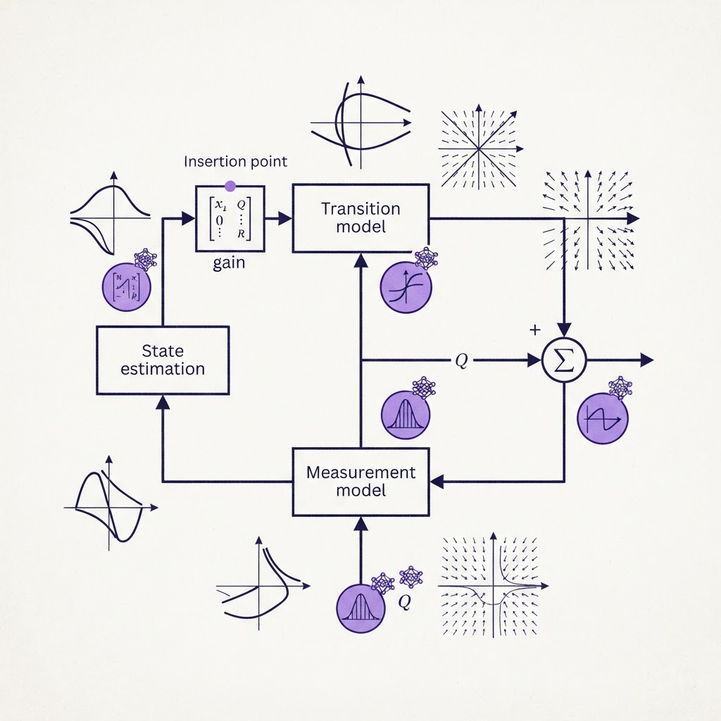
A Kalman filter and neural network hybrid state estimation scheme is what you build when the filter you have is drifting and the network you could train instead would leave you with no covariance, no interpretability and no argument for a safety case. The literature on these hybrids is now two decades deep and almost entirely written for signal-processing peers. What it lacks is a map: where in the filter the network goes, what each placement keeps of the Kalman guarantees, and what the measured gain has been where somebody bothered to measure it.
This article builds that map from the surveys' own taxonomies, quotes the numbers, and then asks the only question we care about at Equation Labs: which of these architectures survives contact with a living process whose model is incomplete by nature.
Why a filter and a network end up in the same estimator
The AI-aided Kalman filter tutorial from the group that wrote KalmanNet lists what a model-based filter gives you when its state-space model is right: minimum mean-squared error for the linear Gaussian case, controllable and usually small complexity, interpretable internal quantities, natural adaptation when the model changes, and an error covariance delivered alongside every estimate. It then lists what replacing the filter with a deep network costs: a training burden and data appetite that hardware-limited devices cannot carry, opacity about how a prediction was reached, and weak adaptation to distribution shift with no reliable uncertainty. The authors' conclusion is that the productive direction is not replacement but augmentation, with the filter kept as the inductive bias and the network filling in what the model does not know.
That framing is recent, the practice is not. The 2023 review by Feng and colleagues traces hybrid Kalman and neural estimators to pioneering work in 1994 and sorts the field into three structural types: filter and network used in succession, a network whose parameters are trained by the filter, and a filter whose equations or parameters are supplied by the network. Their reading of the evidence is that hybrids outperform either component alone in both accuracy and generalisation, with the honest caveat that application to practical problems is still at an early stage and the filter-informed-by-network family is the emerging one.
Four places a neural network can enter the Kalman filter
The most useful taxonomy for a practitioner is the one in the Cranfield review of 55 papers, because it sorts by the role the network plays rather than by the type of network. Of the 55, 31 percent tune filter parameters, 25 percent compensate the filter's error, 27 percent update the state vector or the measurements, 13 percent manufacture pseudo-measurements and 4 percent combine groups. Two open issues the reviewers call out apply to everything below: most papers validate weakly against prior methods, and almost none report computational complexity.
Tuning the noise covariances
The process and measurement noise covariances are the two matrices every Kalman user tunes by hand and then leaves constant. The Cranfield review finds that this group mostly pairs an adaptive extended Kalman filter with a feedforward or recurrent network that takes the innovation, the gap between predicted and actual measurement, as its input and outputs the covariances. The filter's equations are untouched. The network only decides how much to trust the model versus the sensor at each step, which is exactly the decision a fixed covariance gets wrong when the environment changes.
Compensating the filter's error
The second group trains a network to predict the residual between the filter's estimate and the truth, then adds it on. The review notes this is usually a linear Kalman filter plus a backpropagation network, chosen for simplicity, and that the simplicity is why it appears in so many applications. The filter still runs as designed. The network is a post-processor that absorbs unmodelled error, which also means its correction carries no covariance of its own.
Replacing the part of the model you do not have
The third placement puts the network inside the state-space model, as the transition function, the measurement function, or one term of either. A 2024 study in Electronics used a physics-informed network trained with a combined data and physics loss as the transition model of an unscented Kalman filter, propagating the sigma points through the network, adapting the noise covariances online, appending model parameters to the state vector and using Monte Carlo dropout for uncertainty. The filter's moment recursion is preserved. What changes is that the function it differentiates or samples is learned. This is the family our own work sits in, and we return to it below.
Learning the gain itself
The fourth placement is the most invasive. KalmanNet keeps the prediction and update flow of the filter but replaces the Kalman gain computation with a recurrent network. Because the gain is the only place the noise statistics and the covariance propagation enter, learning it sidesteps the need to know those statistics, removes the per-step matrix inversion, and removes the linearisation the extended filter relies on. The authors demonstrate that with full model information KalmanNet coincides with the classical filter, which is the sanity check any hybrid should pass.
What the measured gains look like
KalmanNet's numbers are the clearest in the field because every experiment pairs it against a model-based filter with the same partial information. Under a state-evolution mismatch, KalmanNet achieved a 3 dB gain over the Kalman filter and landed within a minor gap of the minimum mean-squared error, the number a filter with the true model would reach. Under a 10 degree rotation of the observation matrix, about 5 percent sensor misalignment, it converged near the same bound. On a nonlinear synthetic model the extended Kalman filter degraded at high observation noise and KalmanNet did not. It was trained on trajectories of 100 steps and tested on trajectories of 1000, and a fully model-agnostic recurrent network trained on the same task diverged. The alphaXiv summary of the paper records the real-data result, 22.2 dB against 25.4 dB for the Kalman filter on the Michigan NCLT localisation set, and the timing on the Lorenz benchmark: 4.7 seconds for KalmanNet, 5.4 for the extended Kalman filter and 63 for a particle filter. The learned gain was not the slow option.
The stronger recent number comes from Unscented KalmanNet, which augments the unscented filter with two bounded learned corrections and reports RMSE reductions against the plain unscented filter of 26.4 to 49.7 percent on synthetic systems, and 22.4 and 34.3 percent in position and velocity across 11 real flights under leave-one-sequence-out validation. That study matters for a reason beyond the percentages, covered next.
What each architecture keeps of the Kalman guarantees
The covariance is the thing you lose first
The Unscented KalmanNet authors say plainly what earlier work left implicit: existing learned filters either forgo an explicit covariance or learn an uncertainty without correcting the gain bias that model mismatch introduces, so the reported posterior stops being consistent with the actual error. Their fix is instructive because it is structural rather than statistical. One module predicts time-varying process and measurement covariances as bounded multiplicative corrections to fixed baselines, which keeps both matrices positive definite by construction. A second applies a bounded residual correction to the analytical gain, so the sigma-point moment structure is never discarded. A calibration-aware loss adds covariance and innovation-consistency terms to the state error. The result had normalised estimation error squared and empirical coverage closest to nominal among the filters compared. In other words, the network was allowed to move the filter, but only inside a box the filter's theory defines.
A decision table
| Where the network goes | What stays analytical | What is learned | What you must check |
|---|---|---|---|
| Noise covariances | Entire recursion, covariance output | Trust between model and sensor per step | Covariances stay positive definite; innovation whiteness |
| Error compensation | Entire recursion | Residual after the filter | The correction has no covariance; bound its magnitude |
| Model component | Moment propagation, update | Transition or measurement function | Estimability of the states the network feeds; sigma-point or Jacobian cost of the network |
| Kalman gain | Prediction and update flow | The gain | Coincides with the filter under full information; covariance only if explicitly restored |
Read from top to bottom, each row buys more robustness to model mismatch and gives up more of the covariance story. The right row is the lowest one that fixes the failure you actually observed, not the most powerful one.
On a living process: the hybrid that has run on real cultivation data
Balances in the filter, learning in the observation model
The one hybrid Kalman estimator in this literature that ran on real cultivation data is the Simutis and Luebbert study on a recombinant protein process in E. coli. Their design decision is the whole lesson. The state model stayed as ordinary differential equations from mass balances on biomass, substrate and product, because those balances are reliable. The observation model, the mapping from the only online signals available, cumulative oxygen uptake and carbon dioxide production rates, to biomass and product concentration, was learned, because the textbook relations for it are not accurate enough. The specific growth rate was appended to the state vector and estimated alongside the concentrations. The filter was an unscented one, which uses both models directly with no linearisation. The authors also recorded why they did not reach for a particle filter: its small accuracy gain does not justify its computational expenditure in biotechnology.
When the mechanistic model is incomplete
That split, physics where it is trustworthy and learning where it is not, has a 30 year pedigree in bioprocess modelling. The Fermentation review of hybrid bioprocess models summarises the Psichogios and Ungar comparison of 1992, which placed a feedforward network in series with balance equations for a fed-batch bioreactor and tested it against extended Kalman filtering and nonlinear programming. With a detailed mechanistic model available, the extended Kalman filter and the optimisation estimator won. With an incomplete or unreliable mechanistic model, the hybrid won, generalised better, and was easier to interpret than a fully neural model. Every cultivation we have worked on is the second case.
The modern form of that series structure is the physics-informed network, where the balance equations enter the loss rather than sit beside the network. The Jülich and TU Delft study on process operations with limited knowledge and data notes that Kalman filtering has recently been combined with such networks, and shows that a physics-informed network can infer states that have neither a sensor nor a constitutive equation, with a heuristic to test estimability before you commit. We cover that test and the bioprocess results in our article on physics-informed neural networks for state estimation in bioprocesses.
What we run on a 500 L pilot basin
Our stack in the OptiVX programme follows the Simutis split rather than the KalmanNet one, for the reasons the decision table gives. The growth model is a physics-informed network whose accuracy reached an R-squared above 0.95 on the 500 L pilot basin. It sits inside the estimator as the model component; the filter's moment propagation and update are left as the theory wrote them, so the covariance that the next layer consumes is a real one. That next layer is a safety filter that runs in under 2 ms, and it is the reason we will not accept a learned gain without a restored covariance: a barrier function needs an error bar it can trust. End-to-end edge latency was brought from 1.2 seconds to 285 ms, and over 400 simulated years of operation the safety layer recorded zero violations. The latency figure is what decides how large the network inside the filter may be, which is a compression problem we treat in our piece on edge AI model compression, and the identification of the network itself is the subject of neural ordinary differential equations for nonlinear system identification.
Two features of a cultivation push the choice further. States cannot go negative and measurements arrive on different clocks, and neither the Kalman recursion nor a learned gain has a natural place for a hard bound. Where that dominates, the filter gives way to an optimisation over a window, a comparison we make in moving horizon estimation vs Kalman filter. How the estimate then feeds the controller is set out in our bioreactor control strategy.
A build order
- Run the plain filter with the best mechanistic model you have and log the innovation sequence. If the innovations are white and the covariance is consistent, stop. The basics of that recursion are in Kalman filter for state estimation.
- If the innovations are coloured but the state is tracked, learn the noise covariances from the innovation. Constrain the output to positive definite corrections of a baseline.
- If the state drifts with a repeatable bias, learn the residual and bound its magnitude. Treat the correction as a diagnostic that tells you which part of the model is wrong.
- If one function in the model is simply unknown, learn that function, keep the balances, and test estimability of every state the network feeds before training.
- Only if the model is wrong in ways you cannot localise, learn the gain, and insist on the full-information sanity check and an explicitly restored covariance before a controller is allowed to act on the estimate.
- If hard bounds or multi-rate measurements dominate the failure, you have left Kalman territory. The options are compared in Kalman filter alternatives.
FAQ
Does a hybrid Kalman neural network estimator still give an error covariance?
It depends on where the network sits. Covariance tuning, error compensation and model-component hybrids leave the analytical covariance recursion in place. A learned gain in the KalmanNet style forgoes an explicit covariance unless it is restored, which Unscented KalmanNet does with bounded positive-definite corrections and a calibration term in the loss.
How much training data does a learned Kalman gain need?
Less than a free-standing network. KalmanNet was trained on trajectories of 100 steps and tested on trajectories of 1000, converged much faster than purely data-driven recurrent networks, and the model-agnostic network trained on the same task diverged.
Is a hybrid estimator slower than an extended Kalman filter at run time?
Not necessarily. A learned gain skips the Jacobians and matrix inversions the extended filter performs at every step, and on the Lorenz benchmark KalmanNet inferred in 4.7 seconds against 5.4 for the extended filter and 63 for a particle filter on the same hardware. A network used as the transition model costs more, because sigma points or Jacobians are propagated through it.
Should the network replace the process model or the measurement model in a bioreactor?
The measurement model, in the one study on real cultivation data. The mass balances for biomass, substrate and product were kept as the process model because they are reliable, and the relation from off-gas rates to concentration was learned because it is not.