
Domain randomization is the standard answer to sim to real transfer, and almost every published account of it is an account of a robot. Randomise mass, friction, actuator gains and camera pose across a few thousand parallel rollouts, and the policy stops depending on the particular simulator it was trained in.
The method generalises. The recipes do not. A gasifier, a distillation column or a cultivation basin has no textures to randomise, resets on the timescale of the process rather than in seconds, and reports its state through analysers that drift. This article takes the method apart and rebuilds its inputs for that setting: which factor classes survive the move, where the ranges legitimately come from, and why the adaptive variants that dominate the literature are mostly unavailable to you.
What domain randomization assumes before it does anything
The canonical review of robot learning from randomized simulations gives the definition worth working from. The common characteristic of these approaches is the perturbation of simulator parameters, state observations, or applied actions. Randomization is a regularizer: it stops the learner overfitting to individual simulation instances, and from a Bayesian view the distribution over simulators is a representation of your uncertainty about the real one.
That last sentence is the whole design brief. If the distribution represents your uncertainty, then setting it carelessly is not conservatism, it is lying about what you know.
The same review states the premise that makes randomization necessary at all: there is a consensus that further increasing the simulator's accuracy alone will not bridge the gap. And it names the assumption underneath, by listing what gets randomised. Inertia and geometry, friction and contact models, actuation delays, motor efficiency coefficients, sensor noise levels, colours, illumination, camera pose. Every item is a number a physics engine already holds. You can only randomise a factor your simulator has a parameter for, which means the method's reach is exactly the reach of your model.
The four factor classes, and the two that barely exist on a plant
The most useful practitioner framing splits randomization into four factor classes: visual, physics, sensor and task, and warns against the characteristic error of randomising visual factors when the real problem is contact. Map those four onto a process and two of them collapse.
Visual is empty. There is no camera in the loop, so the entire literature on textures, glare and lighting is inapplicable rather than merely less important. Task randomization thins out too: a manipulator faces a new object pose every episode, while a plant runs a setpoint programme that changes on the scale of campaigns.
What is left carries the whole budget, and it is not shaped like rigid-body physics.
Physics becomes kinetics and initial conditions
The bioprocess literature is the one place this has been worked out in the open. A study applying domain randomization to dynamic metabolic control in E. coli randomises exactly two things, and the reasoning behind each is the transferable part. Initial conditions are randomised to capture measurement error and variability in growth media or inoculum. Kinetic parameters are randomised to capture intrinsic stochastic phenomena, external disturbances such as temperature, pH and mixing variability, and wrong or oversimplified model assumptions.
Note what the second category admits. Randomising a kinetic coefficient is being used as a proxy for model error, not only for genuine physical variation. That is a defensible move and an underdeclared one, and it belongs in your documentation as such.
Sensor randomization is where a slow process actually spends
On a robot the encoder is close to ground truth. On a plant the state is inferred, and the inference degrades between calibrations. Analyser lag, zero drift, a probe fouling over a campaign and a lab assay arriving four hours after the sample: these are the perturbations most likely to break a transferred policy, and they have no analogue in a manipulation benchmark.
The practical rule from the same four-class treatment still applies, and matters more here: sample coupled factors together rather than independently. A drifting temperature probe changes both the reading and the reaction rate the controller is reacting to. Sampling those two independently generates episodes that cannot physically occur, and the policy spends capacity learning to handle them.
Where the ranges come from
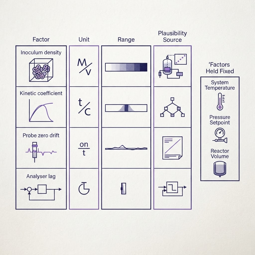
This is the question the ranking pages leave unanswered, and the answer is procedural rather than clever. Every randomised factor needs four things written down: a unit, a range, a distribution, and a plausibility source. The fourth is the one that does the work. On a process the legitimate plausibility sources are narrow: the instrument specification sheet, the spread across historical batch records, and the residuals from your own parameter identification. Intuition is not one of them.
Distribution follows from the source. The bioprocess work above uses Gaussians around nominal values and says explicitly that alternatives may be used based on prior knowledge, and the journal version of that framework is blunt about the provenance: the probability distributions are built on domain knowledge or empirical data. Where you have a measured spread, use it. Where you only have bounds from a datasheet, uniform between the bounds is the honest choice.
Where no source exists, the useful move is to stop treating the range as a fixed decision. The same study sweeps the uncertainty level across 0, 10, 15, 20 and 25 percent and reports how the policy degrades, which converts an unjustifiable guess into a designed experiment whose output is a robustness curve. That study is also the strongest available evidence that this pays outside robotics: its randomised dynamic policies achieved up to 40 percent higher titers than static control while remaining robust under uncertainty. And it needs only forward integration of the model, which is why it is proposed as an alternative to stochastic MPC rather than an approximation of it.
Wider is not safer
The instinct, once ranges become uncomfortable, is to widen them. It does not work that way, and there is a clean demonstration.
SimOpt, the reference method for adapting randomization from real data, was tested on a drawer whose position in the target scene was offset by 15 cm and 22 cm. The authors note that covering that offset by naive randomization would have required a standard deviation of at least 10 cm on the cabinet position, and that this fails to produce a policy that opens the drawer at all. Starting from a conservative distribution and adapting it took three iterations for the 15 cm case and five for 22 cm. A distribution wide enough to guarantee the truth is inside it is frequently too wide to learn anything from, because most of its mass describes situations that do not occur.
The theory agrees, in a form worth knowing. Work on the conditions under which domain randomization provably works models the simulator as a set of MDPs with tunable parameters and proves that transfer can succeed without any real-world training samples, with a sim-to-real gap that is sublinear in the horizon when the randomised simulator class is finite or satisfies a smoothness condition. The same paper supplies a lower bound showing that those benign conditions are necessary, not merely convenient. A wide, rough, discontinuous family of simulators is outside the regime where the guarantee exists.
One more result from that analysis deserves to survive into practice: memory matters. History-dependent policies, not just state-feedback ones, are what let an agent identify which environment it is in from the trajectory so far. On a process where the unmeasured drift only reveals itself over hours, that is the difference between a controller that adapts and one that averages.
Adaptive randomization, and why the online versions do not fit a plant
The literature's answer to hand-tuned ranges is to learn them. BayRn puts the objection to static distributions plainly: they are set by trial and error, and a fixed distribution assumes prior knowledge about the uncertainty that you may not have. It replaces the guesswork with Bayesian optimisation over the distribution parameters, scored on real-system returns.
The catch is the scoring. A benchmark of adaptive domain randomization methods splits the field by data requirement. Online methods including SimOpt and BayRn iteratively roll out the current policy on the target system and adapt from what comes back, and their performance is limited by the quality of that intermediate policy. Offline methods work from a fixed dataset and, in the benchmark, gave better jump-start performance with fewer target transitions available. BayRn's Gaussian process needs roughly five to ten real evaluations before its posterior means anything.
Now put that against the data reality of a slow process. In biomanufacturing it is very common to work with 3 to 20 process observations, and personalised therapies force R&D to work with 3 to 5 batches. Ten real evaluations is not a modest requirement in that setting, it is more experiments than the programme has.
So the online branch is closed, and the choice is between offline adaptation from whatever historical record exists, and calibrating the simulator rather than widening it. The second is an active line: an actor-simulator framework calibrates a digital twin and searches for the control policy jointly, tested with up to 40 unknown calibration parameters in a biopharmaceutical setting, choosing the next experiment to maximise uncertainty while penalising high-uncertainty actions in the policy itself. Randomising a parameter and identifying it are not rivals. Identify what the data supports, randomise the residual, and say which is which. That argument is the same one for a digital twin good enough to certify against, and it starts with a state model that derives the dynamics rather than fits the output.
The factors you cannot randomise
Randomization covers parametric mismatch. It does nothing about a phenomenon your model does not represent, which on a plant is the ordinary case and the subject of the reality gap on a live process.
Two architectural responses, and they compose. The first is staged training: train the policy offline on a preliminary mechanistic model, then adapt on the true plant with transfer learning, retraining only the last hidden layers so that a handful of real batches cannot push a deep network into a bad local optimum or divergence. The second is a runtime layer that holds regardless of what the policy learned, because a control barrier function turns that into a hard constraint rather than a trained tendency. Randomization buys robustness in distribution. The safety layer is what covers the tail you never sampled, and it is also what makes the question of when zero shot transfer is defensible answerable at all.
What a randomization record has to state
The deliverable is not the policy. It is the statement of what was varied and what was held still.
Ours reads as a table with four columns, the fourth being the plausibility source, and a second list of the factors deliberately left fixed with the reason for each. Around it sit the measured figures from our own control stack: growth-model accuracy at R-squared above 0.95, validation on a 500 L pilot basin with zero safety violations across 400 simulated years, and on the OptiVX programme 29 accounted work phases with those 400 simulated years certified.
We say the same thing about that number every time it appears, because it is the part most easily misread. Four hundred simulated years is coverage of the state space, not elapsed operating time, and it is worth exactly as much as the randomization ranges that generated it. A simulator agreeing with itself across a narrow distribution for four hundred years proves that the distribution was narrow. The record is what turns coverage into evidence, and the same discipline decides choosing a bioreactor control strategy before any of it reaches an actuator.
FAQ
How wide should the randomization ranges be?
Wide enough to cover the plausible range of the factor as your instrument or your batch history measures it, and no wider. Widening a distribution until it certainly contains the truth is a known failure mode: covering a 15 cm positional offset by naive randomization was calculated to need a 10 cm standard deviation and produced a policy that could not do the task, whereas starting conservative and adapting from real data solved it in three iterations.
Does domain randomization work with no real-world data at all?
Provably yes, but conditionally. The sim-to-real gap is bounded sublinearly in the horizon when the randomised simulator class is finite or satisfies a smoothness condition, and the accompanying lower bound establishes that those conditions are necessary rather than a proof convenience. The same analysis shows that policies with memory do better than memoryless ones under randomization, because the trajectory itself identifies which environment the agent is in.
What distribution should I sample from?
Whatever your plausibility source supports. Gaussian around a nominal value when you have a measured spread, uniform between bounds when a datasheet gives you only bounds. The published bioprocess implementations use Gaussians on initial conditions and kinetic parameters by default and state explicitly that other distributions may be used given prior knowledge of the uncertainty.
Should I randomise a parameter or identify it?
Both, in that order. Identify what your data supports, then randomise the residual uncertainty. Recent work does the two jointly, calibrating a digital twin while searching for the policy across as many as 40 unknown parameters, and choosing each next experiment to attack the largest remaining uncertainty.
Can I use domain randomization with only a few batches of data?
Yes, but not the online adaptive variants. Those need repeated rollouts of the current policy on the real system, roughly five to ten before the search is even informative, and biomanufacturing commonly works with 3 to 20 process observations in total. With that budget the ranges have to come from instrument specifications and historical batch records, with any adaptation done offline against data you already hold.